Chapter 36Electric Potential and Capacitors

Example 36.1: Work received by a charge in a uniform electric field

In a uniform electric field of magnitude $E=2.0\times10^3\ \mathrm{N/C}$, a point charge $q=4.0\ \mu\mathrm C$ moves a distance $d=0.50\ \mathrm m$ in the same direction as the field. (1) Find the potential difference $\varphi_B-\varphi_A$ between the starting point $B$ and the arrival point $A$. (2) Find the work $W_{BA}$ done on the charge by the electric field.

Solution. (1) In a uniform electric field, the potential difference between two points a distance $d$ apart along the direction of the field is $\varphi_B-\varphi_A=Ed$ by Eq. \eqref{eq:36-uniform-V}, which we will derive in Section 36.2 (here we anticipate the result and calculate numerically).

$$ \varphi_B-\varphi_A=Ed=(2.0\times10^3\ \mathrm{N/C})\times(0.50\ \mathrm m)=1.0\times10^3\ \mathrm V $$

(Unit check: $\mathrm{N/C}\times\mathrm m=\mathrm{N\cdot m/C}=\mathrm{J/C}=\mathrm V$, which agrees with the unit of the potential difference.)

(2) By Eq. \eqref{eq:36-work-potdiff},

$$ W_{BA}=q(\varphi_B-\varphi_A)=(4.0\times10^{-6}\ \mathrm C)\times(1.0\times10^3\ \mathrm V)=4.0\times10^{-3}\ \mathrm J=4.0\ \mathrm{mJ} $$

(Unit check: $\mathrm{C\cdot V}=\mathrm{C\cdot(J/C)}=\mathrm J$.)

Example 36.2: Potential around a point charge

For a point charge carrying $Q=2.0\ \mathrm{nC}$ of electric charge, find the potential $\varphi(r_A)$ at a point $A$ at distance $r_A=5.0\ \mathrm{cm}$ from the charge and the potential $\varphi(r_B)$ at a point $B$ at distance $r_B=15\ \mathrm{cm}$, and then find the potential difference $\varphi(r_A)-\varphi(r_B)$. You may use the Coulomb constant $k=\dfrac{1}{4\pi\varepsilon_0}\approx8.99\times10^9\ \mathrm{N\cdot m^2/C^2}$.

Solution. By Eq. \eqref{eq:36-point-charge-potential},

$$ \varphi(r_A)=k\frac{Q}{r_A}=(8.99\times10^9)\times\frac{2.0\times10^{-9}}{5.0\times10^{-2}}\ \mathrm V\approx3.6\times10^2\ \mathrm V $$ $$ \varphi(r_B)=k\frac{Q}{r_B}=(8.99\times10^9)\times\frac{2.0\times10^{-9}}{15\times10^{-2}}\ \mathrm V\approx1.2\times10^2\ \mathrm V $$ $$ \varphi(r_A)-\varphi(r_B)\approx3.6\times10^2-1.2\times10^2=2.4\times10^2\ \mathrm V $$

(The potential is higher at $A$ because it is closer to the charge. This corresponds to the fact that positive work must be done from outside to bring a positive charge closer from $B$ to $A$.)

Example 36.3: Electrostatic potential energy of the electron and proton in a hydrogen atom

In Chapter 35, we saw that the Coulomb force between an electron and a proton is about $10^{39}$ times the gravitational attraction between the same two particles. How large, then, is the electrostatic potential energy in an actual hydrogen atom (a model in which the electron and proton are taken to be separated by the Bohr radius $a_0\approx5.29\times10^{-11}\ \mathrm m$)? Calculate it using the elementary charge $e=1.602\,176\,634\times10^{-19}\ \mathrm C$, and give the answer both in the unit $\mathrm J$ and in the unit $\mathrm{eV}$ (the electronvolt, $1\,\mathrm{eV}=e\times1\,\mathrm V=1.602\times10^{-19}\ \mathrm J$), which is commonly used for the energies of atoms and molecules.

Solution. The charge of the electron is $-e$ and that of the proton is $+e$, so setting $q=-e,\ Q=+e,\ r=a_0$ in Eq. \eqref{eq:36-two-charge-pe}, we obtain

$$ U=\frac{1}{4\pi\varepsilon_0}\frac{(-e)(e)}{a_0}=-\frac{1}{4\pi\varepsilon_0}\frac{e^2}{a_0} $$

Substituting the numerical values gives

$$ U=-(8.99\times10^9)\times\frac{(1.602\times10^{-19})^2}{5.29\times10^{-11}}\ \mathrm J\approx-4.36\times10^{-18}\ \mathrm J $$

Converting to electronvolts gives

$$ U\approx\frac{-4.36\times10^{-18}\ \mathrm J}{1.602\times10^{-19}\ \mathrm{J/eV}}\approx-27.2\ \mathrm{eV} $$

The negative sign indicates that the electron and proton attract each other, so energy must be supplied from outside to pull them apart. Interestingly, the ground-state energy of the hydrogen atom obtained from quantum mechanics is known to be $-13.6\ \mathrm{eV}$, which is exactly half of this electrostatic potential energy (in absolute value)—a manifestation of the general property that, under a force of the $1/r$ type such as the Coulomb force, the total energy of a bound state is exactly half of the potential energy (the virial theorem). Even from the classical electrostatics calculation of this chapter alone, one can correctly estimate that the energy scale of atoms is of the order of magnitude of $\mathrm{eV}$.

Example 36.4: Electric field of an infinitely wide charged plane

Charge is distributed with uniform surface charge density $\sigma\,[\mathrm{C/m^2}]$ on an infinitely wide flat plate. Find the magnitude of the electric field that this plate creates around it.

Solution. Choose a cylinder (the Gaussian surface) whose axis is perpendicular to the plane, so that it is symmetric about the plane. Let the areas of its top and bottom faces each be $S$ (Figure 36.3). By symmetry, the electric field is perpendicular to the plane (along the axis of the cylinder) and has the same magnitude $E$ on both the top and bottom faces. Moreover, since the electric field points along the axis of the cylinder, it is parallel to the side surface, which is parallel to the axis (perpendicular to the normal vector of the side surface, so that $\bm E\cdot\bm n\,\dd S=0$), and no electric field lines pass through the side surface. Therefore the left-hand side of Gauss's law (the closed-surface integral of the electric field) receives contributions only from the top and bottom faces:

$$ \oint\bm E\cdot\bm n\,\dd S=\underbrace{E\cdot S}_{\text{top}}+\underbrace{E\cdot S}_{\text{bottom}}=2ES $$

The $Q_{\text{enc}}$ on the right-hand side is the charge on the part of area $S$ that the cylinder cuts out of the plane, so $Q_{\text{enc}}=\sigma S$. Hence Gauss's law becomes

$$ E\cdot2S=\frac{\sigma S}{\varepsilon_0} $$

Since the $S$ on both sides cancel, we obtain

\begin{equation} E=\frac{\sigma}{2\varepsilon_0} \label{eq:36-infinite-plane-E} \end{equation}

This does not depend at all on the distance $x$ from the plane—it is a result that runs counter to intuition but follows necessarily from symmetry: the electric field produced by an infinitely wide plane does not weaken no matter how far one moves away from the plane.

Example 36.5: Electric field of an infinitely long charged line

Charge is distributed with uniform linear density $\delta\,[\mathrm{C/m}]$ along an infinitely long straight line. Find the magnitude of the electric field produced around this line, at a point at perpendicular distance $r$ from the line.

Solution. Consider a cylinder (the Gaussian surface) of radius $r$ and length $\ell$ whose axis is the line (Figure 36.4). By symmetry, the electric field is radial with respect to the line (perpendicular to the side surface of the cylinder, along the radial direction) and has the same magnitude $E(r)$ everywhere on the side surface. On the top and bottom faces of the cylinder, the electric field is parallel to the faces (perpendicular to their normals), so there is no component of the field passing through the faces. Therefore the left-hand side of Gauss's law receives contributions only from the side surface. The area of the side surface is the product $2\pi r\ell$ of the circumference $2\pi r$ of the base and the height $\ell$ (the formula for the lateral area of a cylinder), so the left-hand side is

$$ \oint\bm E\cdot\bm n\,\dd S=E(r)\cdot2\pi r\ell $$

The $Q_{\text{enc}}$ on the right-hand side is the charge on the part of length $\ell$ that the cylinder cuts out of the line, so $Q_{\text{enc}}=\delta\ell$. Hence,

$$ E(r)\cdot2\pi r\ell=\frac{\delta\ell}{\varepsilon_0} $$

Since the $\ell$ on both sides cancel, we obtain

\begin{equation} E(r)=\frac{\delta}{2\pi\varepsilon_0 r} \label{eq:36-infinite-line-E} \end{equation}

Unlike the case of the infinite plane (Eq. \eqref{eq:36-infinite-plane-E}), here the field weakens with the distance $r$ (in proportion to $1/r$). Taken together with the facts that the electric field of a point charge goes as $1/r^2$ and that of an infinite plane is independent of $r$ ($1/r^0$), it is worth noticing the pattern: “each time the number of dimensions over which the charge extends increases by one, the distance dependence of the electric field becomes one step weaker.”

Example 36.6: Potentials of the infinite plane and the infinite line—where to place the reference point

For the infinite plane of Example 36.4 ($\sigma\gt0$; at a point at distance $x\,(\gt0)$ from the plane, the magnitude of the electric field is $E=\dfrac{\sigma}{2\varepsilon_0}$ and its direction is away from the plane) and the infinite line of Example 36.5 ($\delta\gt0$; the magnitude of the electric field is $E(r)=\dfrac{\delta}{2\pi\varepsilon_0r}$ and its direction is away from the line), what happens if we try to take infinity as the reference of the electric potential ($\varphi_\infty=0$), as we did for a point charge (Section 36.2)? And what happens to the potential if we take the reference at a finite position?

Solution. (1) Taking infinity as the reference. As in Section 36.2, taking a path that goes to infinity along the direction of the electric field (the direction away from the source), we have $\varphi=-\displaystyle\int_\infty^A\bm E\cdot\dd\bm r=\int_A^\infty E\,\dd r'$ ($r'$ is the distance from the plane or the line). For the plane (let $A$ be the point at distance $x$),

$$ \varphi(x)=\int_x^\infty\frac{\sigma}{2\varepsilon_0}\,\dd x'=\lim_{c\to\infty}\frac{\sigma}{2\varepsilon_0}(c-x)=\infty $$

For the line (let $A$ be the point at distance $r$), using $\displaystyle\int\frac{\dd r'}{r'}=\ln r'$,

$$ \varphi(r)=\int_r^\infty\frac{\delta}{2\pi\varepsilon_0r'}\,\dd r'=\frac{\delta}{2\pi\varepsilon_0}\lim_{c\to\infty}\bigl(\ln c-\ln r\bigr)=\infty $$

we find that both diverge and no finite value is determined. The cause is that the charge extends to infinity. For a point charge, $E\propto1/r^2$, so the contribution from far away decreases rapidly and $\displaystyle\int^\infty E\,\dd r$ converges; but for the infinite plane $E$ is constant, independent of distance, and for the infinite line $E\propto1/r$ ($\ln r$ grows without bound as $r\to\infty$), so the integral does not converge.

(2) Taking the reference at a finite position. Since the electric potential is a quantity determined up to an arbitrary constant (Section 36.1), we may choose the reference point freely. We use Eq. \eqref{eq:36-potdiff-lineintegral}, $\varphi(B)-\varphi(A)=\displaystyle\int_B^A\bm E\cdot\dd\bm r$, with $B$ the point $x$ (or $r$) and $A$ the reference point. For the plane, taking the reference point on the plane ($x=0$, $\varphi=0$), we obtain

$$ \varphi(x)-0=\int_x^0\frac{\sigma}{2\varepsilon_0}\,\dd x'=-\frac{\sigma}{2\varepsilon_0}\,x\qquad(x\ge0) $$

(The potential decreases at a constant rate in the direction of increasing $x$. We get $E=-\dd\varphi/\dd x=\sigma/(2\varepsilon_0)$, in agreement with Example 36.4.) For the line, taking the reference point at a point at distance $r_0$ from the line ($\varphi(r_0)=0$), we obtain

$$ \varphi(r)-0=\int_r^{r_0}\frac{\delta}{2\pi\varepsilon_0r'}\,\dd r'=\frac{\delta}{2\pi\varepsilon_0}\ln\frac{r_0}{r}=-\frac{\delta}{2\pi\varepsilon_0}\ln\frac{r}{r_0} $$

(We get $E=-\dd\varphi/\dd r=\dfrac{\delta}{2\pi\varepsilon_0r}$, in agreement with Example 36.5.) Even if the reference point is moved to a different position, only a constant is added to the potential, and neither the electric field nor the potential difference between two points changes.

(Unit check: the unit of $\dfrac{\sigma x}{\varepsilon_0}$ is $\dfrac{(\mathrm{C/m^2})\,\mathrm m}{\mathrm{C^2/(N\,m^2)}}=\mathrm{N\,m/C}=\mathrm V$, and the unit of $\dfrac{\delta}{\varepsilon_0}$ is $\dfrac{\mathrm{C/m}}{\mathrm{C^2/(N\,m^2)}}=\mathrm{N\,m/C}=\mathrm V$; both agree with the unit of electric potential.)

Example 36.7: Electric field and potential of a uniformly charged sphere

Charge is distributed with uniform density $\rho_0\,[\mathrm{C/m^3}]$ inside a sphere of radius $a$ centered at the origin $O$ (the total charge is $Q=\tfrac43\pi a^3\rho_0$). Assuming that the exterior of the sphere is vacuum, find the electric field $E(r)$ and the electric potential $\varphi(r)$ (with infinity as the reference) at distance $r$ from the center, treating $0\le r\le a$ and $r\gt a$ separately. Also confirm that the electric field and potential outside coincide with those of a point charge obtained by collecting the total charge $Q$ at the single point at the center, and, for $\rho_0=7.5\times10^{-8}\ \mathrm{C/m^3}$ and $a=0.10\ \mathrm m$, find $E(a)$, $\varphi(0)$, and $\varphi(a)$.

Solution (electric field). Take the spherical surface of radius $r$ as the Gaussian surface. By spherical symmetry, the electric field points in the radial direction and has the same magnitude $E(r)$ everywhere on the sphere, so Gauss's law becomes

$$ E(r)\cdot4\pi r^2=\frac{Q(r)}{\varepsilon_0} $$

(where $Q(r)$ is the charge inside the sphere of radius $r$).

[1] $0\le r\le a$ (inside the sphere). Since the density is constant, $Q(r)$ is “density × volume of the sphere of radius $r$”: $Q(r)=\rho_0\cdot\tfrac43\pi r^3$ (integrating with the volume element $r'^2\sin\theta\,\dd r'\,\dd\theta\,\dd\phi$ gives the same result: $\rho_0\displaystyle\int_0^r r'^2\dd r'\int_0^\pi\sin\theta\,\dd\theta\int_0^{2\pi}\dd\phi=\rho_0\cdot\dfrac{r^3}{3}\cdot2\cdot2\pi=\tfrac43\pi\rho_0r^3$). Therefore,

$$ E(r)=\frac{Q(r)}{4\pi\varepsilon_0r^2}=\frac{\tfrac43\pi\rho_0r^3}{4\pi\varepsilon_0r^2}=\frac{\rho_0}{3\varepsilon_0}\,r\qquad(0\le r\le a) $$

[2] $r\gt a$ (outside the sphere). The charge contained inside the Gaussian surface is all of the charge of the sphere, $Q=\tfrac43\pi a^3\rho_0$, so

$$ E(r)=\frac{Q}{4\pi\varepsilon_0r^2}=\frac{\rho_0a^3}{3\varepsilon_0}\cdot\frac1{r^2}\qquad(r\gt a) $$

The electric field outside has the same form as that of a point charge with the total charge $Q$ collected at the center. Moreover, at $r=a$ the inside and outside expressions both give $\dfrac{\rho_0a}{3\varepsilon_0}$, so the electric field joins continuously (the electric field is maximal at the surface of the sphere, $r=a$).

Solution (electric potential). Taking infinity as the reference, we have $\varphi(r)=\displaystyle\int_r^\infty E(r')\,\dd r'$.

[2] For $r\gt a$,

$$ \varphi(r)=\int_r^\infty\frac{\rho_0a^3}{3\varepsilon_0}\frac1{r'^2}\,\dd r'=\frac{\rho_0a^3}{3\varepsilon_0}\left[-\frac1{r'}\right]_r^\infty=\frac{\rho_0a^3}{3\varepsilon_0\,r}=\frac{1}{4\pi\varepsilon_0}\frac{Q}{r}\qquad(r\gt a) $$

(In the last equality we used $\dfrac{\rho_0a^3}{3}=\dfrac{Q}{4\pi}$. This agrees with the potential of a point charge, Eq. \eqref{eq:36-point-charge-potential}.)

[1] For $0\le r\le a$, the expression for the electric field switches at $r'=a$, so we split the interval of integration into $[r,a]$ and $[a,\infty)$ (the latter part is exactly the potential outside at $r=a$):

$$ \varphi(r)=\int_r^a\frac{\rho_0}{3\varepsilon_0}\,r'\,\dd r'+\frac{\rho_0a^3}{3\varepsilon_0a}=\frac{\rho_0}{6\varepsilon_0}\left(a^2-r^2\right)+\frac{\rho_0a^2}{3\varepsilon_0}=\frac{\rho_0}{6\varepsilon_0}\left(3a^2-r^2\right)\qquad(0\le r\le a) $$

Numerical values. With $\rho_0=7.5\times10^{-8}\ \mathrm{C/m^3}$, $a=0.10\ \mathrm m$, and $\varepsilon_0=8.854\times10^{-12}\ \mathrm{F/m}$, we obtain

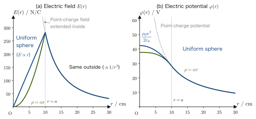
$$ E(a)=\frac{\rho_0a}{3\varepsilon_0}\approx2.8\times10^2\ \mathrm{N/C},\qquad \varphi(0)=\frac{\rho_0a^2}{2\varepsilon_0}\approx42.4\ \mathrm V,\qquad \varphi(a)=\frac{\rho_0a^2}{3\varepsilon_0}\approx28.2\ \mathrm V $$

(Here we used $\varphi(0)=\dfrac{3a^2\rho_0}{6\varepsilon_0}$ and $\varphi(a)=\dfrac{2a^2\rho_0}{6\varepsilon_0}$. The value $\rho_0=7.5\times10^{-8}\ \mathrm{C/m^3}$ was chosen so that the total charge equals that of the sphere in the next Example 36.8 ($\alpha=1.0\times10^{-6}\ \mathrm{C/m^4}$), $Q=\pi\alpha a^4\approx3.1\times10^{-10}\ \mathrm C$. Dimension check: the unit of $\rho_0r/\varepsilon_0$ is $\dfrac{(\mathrm{C/m^3})\,\mathrm m}{\mathrm{C^2/(N\,m^2)}}=\mathrm{N/C}$, which agrees with the unit of the electric field.)

In high school you learned that the electric field is $0$ inside a spherical conducting shell. The sphere here is one (like an insulator) in which the charge is distributed uniformly throughout the volume, and inside it, because the charge enclosed within radius $r$ increases in proportion to $r^3$, the electric field increases linearly in proportion to $r$ from the center to the surface. Outside, even though the charge is spread over the whole sphere, it cannot be distinguished from a point charge (Figure 36.5).

Example 36.8: Electric field and potential of a spherically symmetric charge distribution ($\rho=\alpha r$)

Suppose that charge is distributed inside a sphere of radius $a$ centered at the origin $O$ with density $\rho=\alpha r$ ($\alpha$ is a constant of proportionality; this is a distribution in which the density increases in proportion to the distance $r$ from the center. From the units of $\rho\,[\mathrm{C/m^3}]$ and $r\,[\mathrm m]$, the unit of $\alpha$ is $\mathrm{C/m^4}$). Assuming that the exterior of the sphere is vacuum, find the electric field $E(r)$ and the electric potential $\varphi(r)$ at distance $r$ from the center of the sphere, treating the case $0\le r\le a$ and the case $r\gt a$ separately.

Solution (electric field). Take the spherical surface of radius $r$ as the Gaussian surface. By spherical symmetry, the electric field points in the radial direction and has the same magnitude $E(r)$ everywhere on the sphere, so the left-hand side of Gauss's law (the surface integral) can be written as “magnitude of the electric field × surface area of the sphere,” that is, $E(r)\cdot4\pi r^2$:

$$ E(r)\cdot4\pi r^2=\frac{Q(r)}{\varepsilon_0} $$

Here $Q(r)$ is the total amount of charge contained inside the sphere of radius $r$.

[1] $0\le r\le a$ (inside the sphere). To find $Q(r)$, we integrate the charge density $\rho=\alpha r'$ (to distinguish it from the integration variable, we write the radial coordinate of the point of integration as $r'$) over the whole volume of the sphere from radius $0$ to $r$. The volume element in spherical coordinates is $\dd V=r'^2\sin\theta\,\dd r'\,\dd\theta\,\dd\phi$ (University Mathematics, Section 7.7; for the azimuthal angle we use a different letter, $\phi$, so as not to confuse it with the potential $\varphi$), so

$$ Q(r)=\int_0^{2\pi}\!\!\int_0^\pi\!\!\int_0^r\rho\,r'^2\sin\theta\,\dd r'\,\dd\theta\,\dd\phi=\int_0^{2\pi}\!\!\int_0^\pi\!\!\int_0^r(\alpha r')\,r'^2\sin\theta\,\dd r'\,\dd\theta\,\dd\phi $$

The integrand $\alpha r'^3\sin\theta$ is a product of a “function of $r'$ only,” a “function of $\theta$ only ($\sin\theta$),” and a “constant not containing $\phi$,” so the triple integral separates into a product of three single-variable integrals:

$$ Q(r)=\left(\int_0^r\alpha r'^3\,\dd r'\right)\left(\int_0^\pi\sin\theta\,\dd\theta\right)\left(\int_0^{2\pi}\dd\phi\right)=\left(\frac{\alpha r^4}{4}\right)\times2\times2\pi=\pi\alpha r^4 $$

Therefore,

$$ E(r)\cdot4\pi r^2=\frac{\pi\alpha r^4}{\varepsilon_0}\qquad\therefore\ E(r)=\frac{\alpha r^4}{4\varepsilon_0 r^2}=\frac{\alpha}{4\varepsilon_0}r^2\qquad(0\le r\le a) $$

[2] $r\gt a$ (outside the sphere). Take the spherical surface of radius $r\,(\gt a)$ as the Gaussian surface. The charge contained inside it is just the charge of the entire sphere (radius $a$), $Q(a)=\pi\alpha a^4$ (the result above with $r=a$ substituted), and the region $a\lt r'\lt r$ (vacuum) contains no charge. Therefore,

$$ E(r)\cdot4\pi r^2=\frac{Q(a)}{\varepsilon_0}=\frac{\pi\alpha a^4}{\varepsilon_0}\qquad\therefore\ E(r)=\frac{\alpha a^4}{4\varepsilon_0}\cdot\frac1{r^2}\qquad(r\gt a) $$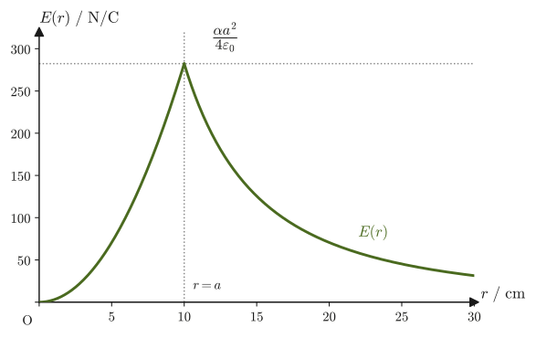

Solution (electric potential). Taking infinity as the reference ($\varphi_\infty=0$), by the same reasoning as for the point charge in Section 36.2 (Eq. \eqref{eq:36-potdiff-lineintegral} with $B=\infty$), we have $\varphi(r)=\displaystyle\int_r^\infty E(r')\,\dd r'$.

[1] For $r\gt a$. Over the whole interval of integration $[r,\infty)$ we need only the expression for the outside, $E(r')=\dfrac{\alpha a^4}{4\varepsilon_0}\dfrac1{r'^2}$ (valid for $r'\gt a$):

$$ \varphi(r)=\int_r^\infty\frac{\alpha a^4}{4\varepsilon_0}\frac1{r'^2}\,\dd r'=\frac{\alpha a^4}{4\varepsilon_0}\left[-\frac1{r'}\right]_r^\infty=\frac{\alpha a^4}{4\varepsilon_0}\left(0+\frac1r\right)=\frac{\alpha a^4}{4\varepsilon_0 r}\qquad(r\gt a) $$

[2] For $0\le r\le a$. Partway through the interval of integration $[r,\infty)$, at $r'=a$, the expression for the electric field switches from the one for the inside to the one for the outside, so we split the interval of integration into the two parts $[r,a]$ and $[a,\infty)$, using the expression for the inside in the first part and the expression for the outside in the second:

$$ \varphi(r)=\int_r^a\frac{\alpha}{4\varepsilon_0}r'^2\,\dd r'+\int_a^\infty\frac{\alpha a^4}{4\varepsilon_0}\frac1{r'^2}\,\dd r' $$

Evaluating each term, we obtain

$$ \int_r^a\frac{\alpha}{4\varepsilon_0}r'^2\,\dd r'=\frac{\alpha}{4\varepsilon_0}\left[\frac{r'^3}3\right]_r^a=\frac{\alpha}{12\varepsilon_0}\left(a^3-r^3\right),\qquad \int_a^\infty\frac{\alpha a^4}{4\varepsilon_0}\frac1{r'^2}\,\dd r'=\frac{\alpha a^4}{4\varepsilon_0}\left[-\frac1{r'}\right]_a^\infty=\frac{\alpha a^3}{4\varepsilon_0} $$

Adding the two and putting them over a common denominator ($\frac14=\frac3{12}$), we get

$$ \varphi(r)=\frac{\alpha}{12\varepsilon_0}\left(a^3-r^3\right)+\frac{3\alpha a^3}{12\varepsilon_0}=\frac{\alpha a^3}{3\varepsilon_0}-\frac{\alpha}{12\varepsilon_0}r^3\qquad(0\le r\le a) $$

(Dimension check: the unit of $\dfrac{\alpha r^2}{\varepsilon_0}$ is $\dfrac{(\mathrm{C/m^4})\,\mathrm{m^2}}{\mathrm{C^2/(N\,m^2)}}=\mathrm{N/C}$, which agrees with the unit of the electric field, and the unit of $\dfrac{\alpha a^3}{\varepsilon_0}$ is $\dfrac{(\mathrm{C/m^4})\,\mathrm{m^3}}{\mathrm{C^2/(N\,m^2)}}=\mathrm{N\,m/C}=\mathrm V$, which agrees with the unit of the electric potential.)

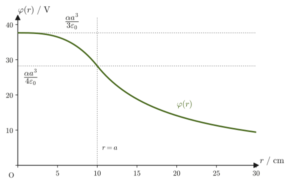
Let us check with numerical values. With $\alpha=1.0\times10^{-6}\ \mathrm{C/m^4}$ and $a=0.10\ \mathrm m$,

$$ E(a)=\frac{\alpha}{4\varepsilon_0}a^2\approx2.8\times10^2\ \mathrm{N/C},\qquad \varphi(0)=\frac{\alpha a^3}{3\varepsilon_0}\approx37.6\ \mathrm V,\qquad \varphi(a)=\frac{\alpha a^3}{4\varepsilon_0}\approx28.2\ \mathrm V $$

(The numerical axes of Figures 36.6 and 36.7 are matched to this example. Since $\varphi(0)\gt\varphi(a)$, the potential is highest at the center and decreases monotonically outward—this is consistent with the electric field always pointing outward (when $\alpha\gt0$).)

Example 36.9: Capacitance, energy, and energy density of a parallel-plate capacitor

A voltage $V=100\ \mathrm V$ is applied to a parallel-plate capacitor with area $S=1.0\times10^{-2}\ \mathrm{m^2}$ (about $10\ \mathrm{cm}\times10\ \mathrm{cm}$) and spacing $d=1.0\ \mathrm{mm}$. Find (1) the capacitance $C$, (2) the electric field $E$ between the plates, (3) the stored electrostatic energy $U$, and (4) the energy density $u$ of the electric field. Also, (5) confirm that the value obtained by multiplying $u$ by the volume $Sd$ between the plates agrees with $U$ in (3).

Solution. (1) By Formula 36.4,

$$ C=\varepsilon_0\frac{S}{d}=(8.854\times10^{-12})\times\frac{1.0\times10^{-2}}{1.0\times10^{-3}}\ \mathrm F\approx8.85\times10^{-11}\ \mathrm F=88.5\ \mathrm{pF} $$

(2) By Eq. \eqref{eq:36-parallel-V},

$$ E=\frac{V}{d}=\frac{100}{1.0\times10^{-3}}\ \mathrm{V/m}=1.0\times10^5\ \mathrm{V/m} $$

(3) By Formula 36.5,

$$ U=\frac12CV^2=\frac12\times(8.85\times10^{-11})\times(100)^2\ \mathrm J\approx4.43\times10^{-7}\ \mathrm J=0.443\ \mu\mathrm J $$

(4) By Formula 36.6,

$$ u=\frac12\varepsilon_0E^2=\frac12\times(8.854\times10^{-12})\times(1.0\times10^5)^2\ \mathrm{J/m^3}\approx4.43\times10^{-2}\ \mathrm{J/m^3} $$

(5) The volume is $Sd=(1.0\times10^{-2})\times(1.0\times10^{-3})=1.0\times10^{-5}\ \mathrm{m^3}$, so

$$ u\times Sd\approx(4.43\times10^{-2})\times(1.0\times10^{-5})\ \mathrm J\approx4.43\times10^{-7}\ \mathrm J $$

This agrees with $U$ in (3) (to within the significant figures). It is a concrete confirmation that $u=\tfrac12\varepsilon_0E^2$ is not a merely formal expression but actually satisfies the relation “volume × density = total energy.”

Example 36.10: Capacitance of a spherical capacitor

A conducting sphere $A$ of radius $a$ is surrounded concentrically by a conducting shell (spherical shell) $B$ of larger radius $b$. When $A$ is given a charge $+Q$ and $B$ is grounded (the potential of $B$ is taken as the reference $0$), find the potential difference between $A,B$ and the capacitance.

Solution. First, let us sort out where the electric field is. When $A$ is given $+Q$, electrostatic induction produces $-Q$ on the inner surface of the conducting shell $B$. Since $B$ is grounded (connected to the earth, so that its potential is held at the reference $0$), the charge on the outer surface of $B$ escapes to the earth, so no charge remains outside $B$ ($r\gt b$) and the electric field there is $0$ as well. The electric field inside the conductor $A$ ($r\lt a$) is also $0$. The electric field differs from $0$ only between $A,B$ ($a\le r\le b$). Therefore, when we integrate the electric field from the center ($r=0$) to infinity, only the portion from $a$ to $b$ among the three intervals contributes (if the potential of $B$ is taken as $0$, the potential difference between $A,B$ is the potential of $A$ itself):

$$ V=\int_0^\infty E(r)\,\dd r=\int_0^a0\,\dd r+\int_a^bE(r)\,\dd r+\int_b^\infty0\,\dd r=\int_a^bE(r)\,\dd r $$

Applying Gauss's law in the region between $A,B$ ($a\le r\le b$), the charge enclosed by a spherical surface of radius $r$ is only the charge $+Q$ of $A$, so by a calculation of the same form as the exterior calculations in Examples 36.7 and 36.8,

$$ E(r)\cdot4\pi r^2=\frac{Q}{\varepsilon_0}\qquad\therefore\ E(r)=\frac{1}{4\pi\varepsilon_0}\frac{Q}{r^2}\qquad(a\le r\le b) $$

(This has the same form as the formula for the electric field of a point charge—it is a manifestation of a general property of Gauss's law: outside a spherically symmetric charge distribution, the electric field can be calculated as if the total charge were concentrated at the center.) The potential difference between $A,B$ is obtained by integrating this electric field from $a$ to $b$, as in the equation above:

$$ V=\int_a^bE(r)\,\dd r=\int_a^b\frac{1}{4\pi\varepsilon_0}\frac{Q}{r^2}\,\dd r=\frac{Q}{4\pi\varepsilon_0}\left[-\frac1r\right]_a^b=\frac{Q}{4\pi\varepsilon_0}\left(\frac1a-\frac1b\right) $$

From $Q=CV$ in Definition 36.4,

$$ Q=C\cdot\frac{Q}{4\pi\varepsilon_0}\left(\frac1a-\frac1b\right)=C\cdot\frac{Q}{4\pi\varepsilon_0}\cdot\frac{b-a}{ab} $$

Canceling $Q$ on both sides and solving for $C$, we obtain

\begin{equation} C=\frac{4\pi\varepsilon_0ab}{b-a} \label{eq:36-spherical-C} \end{equation}

as the capacitance.

Numerical example. With $a=2.0\ \mathrm{cm}$ and $b=5.0\ \mathrm{cm}$, we get $C=\dfrac{4\pi\varepsilon_0\times0.020\times0.050}{0.050-0.020}\approx3.7\times10^{-12}\ \mathrm F=3.7\ \mathrm{pF}$.

Limit of an isolated conducting sphere. If we move the outer shell farther and farther away ($b\to\infty$), we should obtain the capacitance of a single “isolated” conducting sphere with nothing around it. Taking the limit $b\to\infty$ in Eq. \eqref{eq:36-spherical-C},

$$ C=\frac{4\pi\varepsilon_0ab}{b-a}=\frac{4\pi\varepsilon_0a}{1-a/b}\ \xrightarrow[b\to\infty]{}\ 4\pi\varepsilon_0a $$

(We divided the numerator and denominator by $b$ and then let $b\to\infty$, using the fact that $a/b\to0$.) This is exactly the formula “the capacitance of an isolated conducting sphere is $C=4\pi\varepsilon_0a$,” which is often used on its own, and we have confirmed that it follows naturally as a special case of the spherical capacitor (the case in which the radius of the outer shell is made infinite). For example, for an isolated conducting sphere with $a=2.0\ \mathrm{cm}$, $C\approx2.2\times10^{-12}\ \mathrm F=2.2\ \mathrm{pF}$.

Example 36.11: Capacitance of a cylindrical capacitor

A conducting cylinder $A$ of radius $a$ and length $L$ ($L\gg b$) is surrounded by a coaxial conducting cylindrical shell $B$ of radius $b$ ($b\gt a$). When $A$ is given a charge $+Q$ and $B$ is grounded, find the voltage between $A,B$ and the capacitance.

Solution. As with the spherical capacitor, when $A$ is given $+Q$, $-Q$ appears on the inner surface of $B$, and since $B$ is grounded there is no electric field outside $B$. The field inside $A$ is also $E=0$. Because the length $L$ is sufficiently long compared with the radii, the fringing effect at the ends can be neglected, and the electric field is determined only by the distance $r$ from the axis. Therefore, in the voltage as well, only the integral from $a$ to $b$ remains:

$$ V=\int_0^\infty E(r)\,\dd r=\int_0^a0\,\dd r+\int_a^bE(r)\,\dd r+\int_b^\infty0\,\dd r=\int_a^bE(r)\,\dd r $$

Applying Gauss's law in the region between $A,B$ ($a\le r\le b$), by a calculation of the same form as in Example 36.5 (the electric field of an infinite straight line),

$$ E(r)\cdot2\pi rL=\frac{Q}{\varepsilon_0}\qquad\therefore\ E(r)=\frac{Q}{2\pi\varepsilon_0Lr}\qquad(a\le r\le b) $$

The voltage is obtained by integrating this electric field from $a$ to $b$. Using $\displaystyle\int\frac{\dd r}r=\ln r$ (the natural logarithm),

$$ V=\int_a^bE(r)\,\dd r=\frac{Q}{2\pi\varepsilon_0L}\int_a^b\frac{\dd r}r=\frac{Q}{2\pi\varepsilon_0L}\Bigl[\ln r\Bigr]_a^b=\frac{Q}{2\pi\varepsilon_0L}\ln\frac ba $$

From $Q=CV$ we have $Q=C\cdot\dfrac{Q}{2\pi\varepsilon_0L}\ln\dfrac ba$, and canceling $Q$ on both sides, we obtain

\begin{equation} C=\frac{2\pi\varepsilon_0L}{\ln(b/a)} \label{eq:36-cylindrical-C} \end{equation}

as the capacitance.

Numerical example. With $a=1.0\ \mathrm{mm}$, $b=5.0\ \mathrm{mm}$, and $L=0.20\ \mathrm m$ (dimensions close to those of a coaxial cable), we get $C=\dfrac{2\pi\varepsilon_0\times0.20}{\ln5.0}\approx6.9\times10^{-12}\ \mathrm F=6.9\ \mathrm{pF}$.

Relation to the parallel-plate capacitor. Let us consider the limit in which the spacing $t\equiv b-a$ is sufficiently small compared with the radius $a$ ($t\ll a$; the “gap” of the cylindrical shell is thin). Since $\ln(b/a)=\ln(1+t/a)$, and for $t/a\ll1$ the Taylor expansion (University Mathematics, Chapter 4) $\ln(1+x)\approx x$ (the first-order approximation for small $x=t/a$) can be used,

$$ C=\frac{2\pi\varepsilon_0L}{\ln(1+t/a)}\approx\frac{2\pi\varepsilon_0L}{t/a}=\varepsilon_0\frac{2\pi aL}{t} $$

Here $2\pi aL$ is the lateral area of a cylinder of radius $a$ and length $L$ (the surface area of the inner cylinder $A$). If we regard this as the plate area $S$ of a parallel-plate capacitor and the gap $t$ as the plate spacing $d$, the result agrees exactly with $C\approx\varepsilon_0S/d$ (Formula 36.4). This shows that when the gap is thin, even a curved cylindrical surface can be regarded locally as almost flat parallel plates, and it guarantees that Formula 36.4 and Eq. \eqref{eq:36-cylindrical-C} connect consistently.

Example 36.12: Electrostatic energy of a spherical capacitor and the energy density of the electric field

For the spherical capacitor of Example 36.10 ($A$: radius $a$, charge $+Q$; $B$: radius $b$, grounded), find the electrostatic energy by taking the volume integral of the energy density of the electric field $u=\tfrac12\varepsilon_0E^2$ (Formula 36.6) over the whole space between $A,B$, and verify that it agrees with $U=\dfrac{Q^2}{2C}$ of Formula 36.5. Also find $U$ for $a=2.0\ \mathrm{cm}$, $b=5.0\ \mathrm{cm}$, and $Q=1.0\ \mathrm{nC}$.

Solution. The electric field between $A,B$ is $E(r)=\dfrac{Q}{4\pi\varepsilon_0r^2}$, so the energy density is

$$ u(r)=\frac12\varepsilon_0\left(\frac{Q}{4\pi\varepsilon_0r^2}\right)^2=\frac{Q^2}{32\pi^2\varepsilon_0\,r^4} $$

Since $u$ varies from place to place, we add up the energy $u\,\dd V$ stored in a thin spherical shell of radius $r$ and thickness $\dd r$ (its volume is the surface area $4\pi r^2$ times the thickness $\dd r$, that is, $\dd V=4\pi r^2\,\dd r$) from $r=a$ to $r=b$:

$$ U=\int u\,\dd V=\int_a^b\frac{Q^2}{32\pi^2\varepsilon_0r^4}\cdot4\pi r^2\,\dd r=\frac{Q^2}{8\pi\varepsilon_0}\int_a^b\frac{\dd r}{r^2}=\frac{Q^2}{8\pi\varepsilon_0}\left(\frac1a-\frac1b\right) $$

On the other hand, substituting the capacitance, Eq. \eqref{eq:36-spherical-C}, of Example 36.10 into Formula 36.5 gives

$$ U=\frac{Q^2}{2C}=\frac{Q^2}{2}\cdot\frac{b-a}{4\pi\varepsilon_0ab}=\frac{Q^2}{8\pi\varepsilon_0}\cdot\frac{b-a}{ab}=\frac{Q^2}{8\pi\varepsilon_0}\left(\frac1a-\frac1b\right) $$

so the two calculations agree. Even when the electric field varies from place to place, integrating $u=\tfrac12\varepsilon_0E^2$ over the volume gives the correct electrostatic energy.

Numerical values. $\dfrac1a-\dfrac1b=\dfrac1{0.020}-\dfrac1{0.050}=30\ \mathrm{m^{-1}}$ and $\dfrac{Q^2}{8\pi\varepsilon_0}=\dfrac{(1.0\times10^{-9})^2}{8\pi\times8.854\times10^{-12}}\ \mathrm{J\,m}\approx4.49\times10^{-9}\ \mathrm{J\,m}$, so $U\approx4.49\times10^{-9}\times30\ \mathrm J\approx1.3\times10^{-7}\ \mathrm J=0.13\ \mu\mathrm J$. (Using $C=3.7\ \mathrm{pF}$ from Example 36.10, we get $U=\dfrac{Q^2}{2C}=\dfrac{10^{-18}}{2\times3.7\times10^{-12}}\ \mathrm J\approx1.3\times10^{-7}\ \mathrm J$, which agrees.)

Example 36.13: Finding the charge density from Poisson's equation

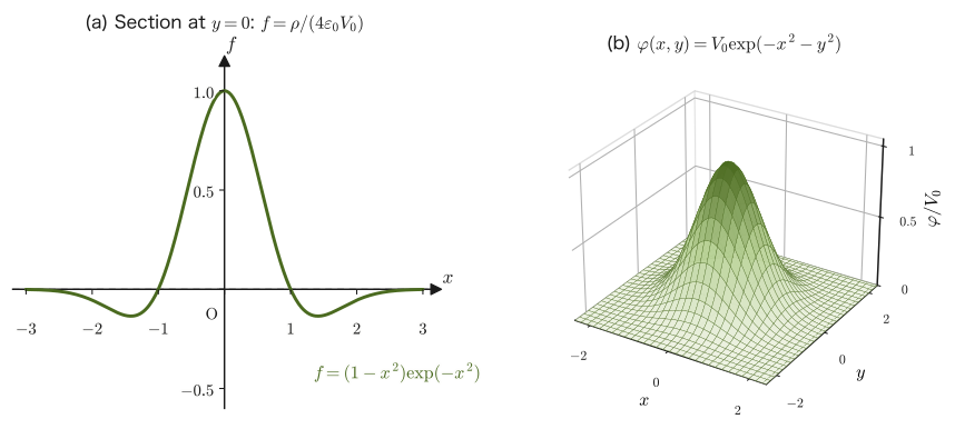
Suppose that the electric potential in some region is given by the function of two variables $\varphi(x,y)=V_0\exp(-x^2-y^2)$ ($V_0\gt0$ is a constant; the distribution rises in a mound shape centered on the origin and does not depend on $z$). Find the charge density $\rho(x,y)$ that produces this potential.

Solution. Since we will use Eq. \eqref{eq:36-poisson}, we first find the second partial derivatives of $\varphi$. Differentiating $\varphi=V_0\exp(-x^2-y^2)$ partially with respect to $x$ (the derivative of a composite function; University Mathematics, Section 6.2), we get

$$ \pdiff{\varphi}{x}=V_0\cdot(-2x)\cdot \exp(-x^2-y^2)=-2xV_0\exp(-x^2-y^2) $$

Differentiating partially with respect to $x$ once more (using the product rule: we differentiate the product of $-2xV_0$ and $\exp(-x^2-y^2)$):

$$ \pdiff{^2\varphi}{x^2}=-2V_0\exp(-x^2-y^2)+(-2xV_0)\cdot(-2x)\exp(-x^2-y^2)=(-2+4x^2)V_0\exp(-x^2-y^2)=(4x^2-2)V_0\exp(-x^2-y^2) $$

Since the function is symmetric in $x,y$, the same calculation for $y$ (simply interchanging $x$ and $y$) gives

$$ \pdiff{^2\varphi}{y^2}=(4y^2-2)V_0\exp(-x^2-y^2) $$

Since $\varphi$ does not depend on $z$, $\pdiff{^2\varphi}{z^2}=0$, and the Laplacian (the sum of the three second partial derivatives with respect to $x,y,z$) reduces to the sum of the two with respect to $x,y$:

$$ \nabla^2\varphi=\pdiff{^2\varphi}{x^2}+\pdiff{^2\varphi}{y^2}=\bigl[(4x^2-2)+(4y^2-2)\bigr]V_0\exp(-x^2-y^2)=4(x^2+y^2-1)V_0\exp(-x^2-y^2) $$

From $\nabla^2\varphi=-\rho/\varepsilon_0$ in Eq. \eqref{eq:36-poisson} we have $\rho=-\varepsilon_0\nabla^2\varphi$, so

$$ \rho(x,y)=-4\varepsilon_0V_0\left(x^2+y^2-1\right)\exp(-x^2-y^2) $$

This is the charge density.

Example 36.14: Potential and field on the axis due to charge on a ring

Charge is distributed uniformly, with linear density $\delta\,[\mathrm{C/m}]$, on a circular loop of radius $a$ (it helps to picture a thin coil-shaped wire). Find the electric potential $\varphi$ and the electric field $E$ at a point $P$ on the central axis of the ring, at distance $x$ from the center.

Solution. We regard the ring as a collection of charge elements $\dd q=\delta\cdot a\,\dd\phi$, each belonging to an infinitesimal arc (of length $a\,\dd\phi$) at azimuthal angle $\phi$ (Figure 36.13; the azimuthal angle is written with a different letter, $\phi$, to distinguish it from the potential $\varphi$). By the symmetry of the ring (its rotational symmetry about the axis), the distance from such a charge element to the point $P$ always has the same value, $r=\sqrt{a^2+x^2}$, regardless of $\phi$ (the hypotenuse of a right triangle whose two legs are the ring radius $a$ and the distance $x$ along the axis). Therefore, applying Eq. \eqref{eq:36-point-charge-potential} to the charge element $\dd q$ and summing (integrating) over the whole ring, we obtain

$$ \varphi=\oint_C\frac{\dd q}{4\pi\varepsilon_0r}=\frac{1}{4\pi\varepsilon_0r}\oint_C\dd q=\frac{1}{4\pi\varepsilon_0\sqrt{a^2+x^2}}\oint_C\delta a\,\dd\phi $$

(the key point is that $r=\sqrt{a^2+x^2}$ is a constant independent of the integration variable $\phi$, so it can be taken outside the integral). Since the charge on one full turn of the ring is $\oint_C\delta a\,\dd\phi=\delta a\displaystyle\int_0^{2\pi}\dd\phi=2\pi a\delta$, we obtain

\begin{equation} \varphi=\frac{2\pi a\delta}{4\pi\varepsilon_0\sqrt{a^2+x^2}}=\frac{\delta a}{2\varepsilon_0\sqrt{a^2+x^2}} \label{eq:36-ring-V} \end{equation}

Next we find the electric field. By symmetry, at a point on the axis only the axial ($x$-direction) component of the electric field remains—this is because the components perpendicular to the axis cancel between paired charge elements on the ring (charge elements on opposite sides of the axis). The axial electric field can therefore be found from $E=-\pdiff{\varphi}{x}$ (the one-dimensional version of Definition 36.1):

$$ E=-\pdiff{\varphi}{x}=-\frac{\delta a}2\pdiff{}{x}\left[(a^2+x^2)^{-1/2}\right]=-\frac{\delta a}2\times\left(-\frac12\right)(a^2+x^2)^{-3/2}\times2x $$

(Derivative of a composite function: when $(a^2+x^2)^{-1/2}$ is differentiated with respect to $x$, the derivative of the outer function, $-\tfrac12u^{-3/2}$ (with $u=a^2+x^2$), is multiplied by the derivative of the inner function, $\pdiff{u}{x}=2x$.) Simplifying, we obtain

\begin{equation} E=\frac{\delta a}{2\varepsilon_0}\cdot\frac{x}{(a^2+x^2)^{3/2}} \label{eq:36-ring-E} \end{equation}

This is the electric field on the axis.

Checking the limits. (i) If $x\gg a$ (far from the ring), then $\sqrt{a^2+x^2}\approx x$, so, writing the total charge of the ring as $Q=2\pi a\delta$, we have $\varphi\approx\dfrac{2\pi a\delta}{4\pi\varepsilon_0x}=\dfrac{Q}{4\pi\varepsilon_0x}$ and $E\approx\dfrac{\delta a}{2\varepsilon_0x^2}=\dfrac{Q}{4\pi\varepsilon_0x^2}$. Seen from far away, the ring is therefore the same as a point charge with the entire charge concentrated at the center (it is also true that $\varphi\to0$ and $E\to0$ as $x\to\infty$). (ii) If $a\to\infty$ (the radius of the ring is made arbitrarily large), the total charge of the ring, $2\pi a\delta$, increases in proportion to $a$, but the distance from each point on the ring to $P$ also increases roughly in proportion to $a$, so Eq. \eqref{eq:36-ring-V} approaches the finite value $\dfrac{\delta}{2\varepsilon_0}$. In this limit $\varphi$ approaches a constant independent of $x$, so the electric field is $E=-\pdiff{\varphi}{x}\to0$ (also by Eq. \eqref{eq:36-ring-E}, $E\approx\dfrac{\delta x}{2\varepsilon_0a^2}\to0$).

Example 36.15: Potential and field on the axis due to charge on a disk

Charge is distributed uniformly, with surface charge density $\sigma\,[\mathrm{C/m^2}]$, on a disk of radius $a$. Find the electric potential $\varphi$ and the electric field $E$ at a point $P$ on the central axis of the disk, at distance $x$ ($x\gt0$) from the center.

Solution. We divide the disk finely using polar coordinates (radius $\ell$, azimuthal angle $\phi$). The charge on the infinitesimal area $\ell\,\dd\ell\,\dd\phi$ at radius $\ell$ ($0\le\ell\le a$) and azimuthal angle $\phi$ is $\dd q=\sigma\ell\,\dd\ell\,\dd\phi$, and the distance from this charge element to the point $P$ is $\sqrt{\ell^2+x^2}$ (Figure 36.14). Summing Eq. \eqref{eq:36-point-charge-potential} (that is, taking a surface integral), we obtain

$$ \varphi=\frac{1}{4\pi\varepsilon_0}\iint\frac{\sigma\,\ell\,\dd\ell\,\dd\phi}{\sqrt{\ell^2+x^2}}=\frac{\sigma}{4\pi\varepsilon_0}\int_0^{2\pi}\!\!\int_0^a\frac{\ell\,\dd\ell}{\sqrt{\ell^2+x^2}}\,\dd\phi $$

The integrand does not depend on $\phi$, so the $\phi$ integral gives $\int_0^{2\pi}\dd\phi=2\pi$, and we obtain

$$ \varphi=\frac{\sigma}{2\varepsilon_0}\int_0^a\frac{\ell\,\dd\ell}{\sqrt{\ell^2+x^2}} $$

This is the same calculation as dividing the disk into thin rings of radius $\ell$ and width $\dd\ell$ (cutting a ring open, we can regard it as a long, thin rectangle of length $2\pi\ell$ and width $\dd\ell$, so its area is $2\pi\ell\,\dd\ell$ and its charge is $\dd q=\sigma\cdot2\pi\ell\,\dd\ell$) and summing, from $\ell=0$ to $a$, the potential that each ring produces at the point $P$ (this is Eq. \eqref{eq:36-ring-V} of Example 36.14 with the replacements $a\to\ell$ and, for the charge of one full turn of the ring, $2\pi a\delta\to\dd q$: $\dd\varphi=\dfrac{\dd q}{4\pi\varepsilon_0\sqrt{\ell^2+x^2}}$). For the remaining integral, the substitution $u=\ell^2+x^2$ gives $\dd u=2\ell\,\dd\ell$, so $\ell\,\dd\ell=\tfrac12\dd u$, and we find $\displaystyle\int\frac{\ell\,\dd\ell}{\sqrt{\ell^2+x^2}}=\int\frac{\tfrac12\dd u}{\sqrt u}=\sqrt u=\sqrt{\ell^2+x^2}$ (an antiderivative). Therefore,

$$ \varphi=\frac{\sigma}{2\varepsilon_0}\Bigl[\sqrt{\ell^2+x^2}\Bigr]_0^a=\frac{\sigma}{2\varepsilon_0}\left(\sqrt{a^2+x^2}-\sqrt{x^2}\right) $$

Since $\sqrt{x^2}=x$ for $x\gt0$, we obtain

\begin{equation} \varphi=\frac{\sigma}{2\varepsilon_0}\left(\sqrt{a^2+x^2}-x\right) \label{eq:36-disk-V} \end{equation}

As in the case of the ring, on the axis only the axial component remains by symmetry, so we find the electric field from $E=-\pdiff{\varphi}{x}$. Using $\pdiff{}{x}\sqrt{a^2+x^2}=\dfrac{x}{\sqrt{a^2+x^2}}$ (derivative of a composite function) and $\pdiff{}{x}(-x)=-1$, we obtain

$$ E=-\pdiff \varphi x=-\frac{\sigma}{2\varepsilon_0}\left(\frac{x}{\sqrt{a^2+x^2}}-1\right)=\frac{\sigma}{2\varepsilon_0}\left(1-\frac{x}{\sqrt{a^2+x^2}}\right) $$

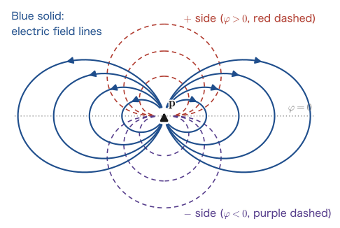
Example 36.16: The electric field produced by the electric dipole moment of a water molecule

A water molecule ($\mathrm{H_2O}$) is charged slightly negatively on the side of the oxygen atom and slightly positively on the side of the two hydrogen atoms, so it can be regarded as an electric dipole. The magnitude of its dipole moment is known from measurements to be approximately $p\approx6.2\times10^{-30}\ \mathrm{C\cdot m}$. Find the potential $\varphi$ and the electric field $E_r$ at a point on the axis of the dipole ($\theta=0$) at a distance $r=1.0\ \mathrm{nm}$ ($=1.0\times10^{-9}\ \mathrm m$, roughly the size of one molecule) from this water molecule.

Solution. Setting $\theta=0$ ($\cos\theta=1$) in Formula 36.8, we obtain

$$ \varphi=\frac{p}{4\pi\varepsilon_0r^2}=(8.99\times10^9)\times\frac{6.2\times10^{-30}}{(1.0\times10^{-9})^2}\ \mathrm V\approx5.6\times10^{-2}\ \mathrm V $$ $$ E_r=\frac{2p}{4\pi\varepsilon_0r^3}=(8.99\times10^9)\times\frac{2\times6.2\times10^{-30}}{(1.0\times10^{-9})^3}\ \mathrm{V/m}\approx1.1\times10^8\ \mathrm{V/m} $$

The potential itself, $0.056\ \mathrm V$, is much smaller than that of a familiar battery (such as $1.5\ \mathrm V$), but because the distance scale is as small as the size of an atom or molecule ($\mathrm{nm}$), the electric field takes the very large value of $10^8\ \mathrm{V/m}$—this estimate shows that one origin of the intermolecular forces that molecules exert on each other (hydrogen bonds and the like) is the electrostatic interaction between dipoles at such extremely short distances.

Example 36.17: Potential and electric field are different quantities—points where $\varphi=0$ and points where $\bm E=\bm 0$

(1) At a point where the potential $\varphi$ is $0$, is the electric field $\bm E$ necessarily $\bm 0$ as well? (2) At a point where the electric field $\bm E$ is $\bm 0$, is the potential $\varphi$ necessarily $0$ as well? For each question, give an example from this chapter that supports your answer.

Solution. In both cases the answer is “not necessarily.” This is because $\bm E=-\nabla\varphi$ expresses the fact that the electric field is determined by the slope of the potential (how much the potential changes from place to place), and has nothing to do with the value of the potential itself.

(1) On the equatorial plane of an electric dipole ($\theta=90°$), Formula 36.8 gives $\varphi=\dfrac{p\cos90°}{4\pi\varepsilon_0r^2}=0$, but the electric field is $E_\theta=\dfrac{p}{4\pi\varepsilon_0r^3}\ne0$. Since the potential changes from positive to negative as we cross the surface where it is $0$, there must be a slope (an electric field) there.

(2) At the center of the ring ($x=0$ in Example 36.14), Eq. \eqref{eq:36-ring-E} gives $E=0$ (this also follows from symmetry: paired charges on the ring cancel each other), but Eq. \eqref{eq:36-ring-V} gives $\varphi=\dfrac{\delta a}{2\varepsilon_0\sqrt{a^2}}=\dfrac{\delta}{2\varepsilon_0}\ne0$. At the center of a uniformly charged sphere (Example 36.7) as well, $E(0)=0$ but $\varphi(0)=\dfrac{\rho_0a^2}{2\varepsilon_0}\ne0$.

The potential is a quantity whose value itself changes with the choice of the reference point (Section 36.1), whereas the electric field is not affected by the choice of reference. The point “$\varphi=0$” moves to a different point depending on the choice of reference, but “$\bm E=\bm 0$” is a physical fact that does not depend on that choice.

Exercise 36.1: Deriving the potential of a point charge from Coulomb's law

Starting from the electric field given by Coulomb's law, $\bm E(r)=\dfrac{1}{4\pi\varepsilon_0}\dfrac{Q}{r^2}\bm e_r$, derive, by carrying out the line integral yourself, the formula for the potential of a point charge with infinity as the reference, $\varphi(r)=\dfrac{1}{4\pi\varepsilon_0}\dfrac Qr$ (Eq. \eqref{eq:36-point-charge-potential}).

Hint: Reproduce on your own, without looking, the calculation carried out in “Derivation: The potential at a point at distance $r$ from a point charge” in Section 36.2. Confirm that the value at the lower limit of the integration interval ($\infty$) vanishes by using the limit $\lim_{c\to\infty}(1/c)=0$.

→ Solution

Exercise 36.2: Two infinite plane charges of opposite signs

An infinite plane with surface charge density $+\sigma$ and a parallel infinite plane with surface charge density $-\sigma$ face each other at a spacing $d$. Using the principle of superposition, find the magnitude and direction of the electric field in each of the regions (1) between the two planes and (2) outside the two planes.

Hint: The idea is the same as when we found the electric field of the parallel-plate capacitor in Section 36.6. The magnitude of the field that each plane produces by itself is $\sigma/(2\varepsilon_0)$, the same as in Example 36.4 (Eq. \eqref{eq:36-infinite-plane-E}). Draw a figure and check, in each of the two regions, whether the contributions from the two planes point in the same direction or in opposite directions.

→ Solution

Exercise 36.3: Equivalent capacitance of capacitors connected in series and in parallel

Derive the equivalent capacitance $C$ obtained when two capacitors of capacitances $C_1,C_2$ are connected (1) in series and (2) in parallel.

Hint: In a series connection, the charge $Q$ stored on each capacitor is the same (conservation of charge), and the total potential difference is the sum of the potential differences of the capacitors, $V=V_1+V_2$. In a parallel connection, the potential difference $V$ across each capacitor is the same, and the total charge is the sum of the charges on the capacitors, $Q=Q_1+Q_2$. Apply $C=Q/V$ of Definition 36.4 to each case and simplify. It is also instructive to compare the results with the formulas for the equivalent resistance of resistors in series and in parallel that you will learn in Section 37.5, and to see which corresponds to which (which formula goes with series? which with parallel?).

→ Solution

Exercise 36.4: A spherical charge distribution whose density decreases linearly from the center to the surface

Charge is distributed inside a sphere of radius $a$ with density $\rho=\rho_0\left(1-\dfrac ra\right)$ ($\rho_0$ is a constant; the density is largest at the center and $0$ at the surface $r=a$). Find the total charge $Q$, and the electric field $E(r)$ and the potential $\varphi(r)$ (with infinity as the reference) at a distance $r$ from the center, treating $0\le r\le a$ and $r\gt a$ separately. Also find the position at which the electric field is maximum and its value there.

Hint: The procedure is the same as in Examples 36.7 and 36.8. Carry out $Q(r)=4\pi\displaystyle\int_0^r\rho(r')\,r'^2\,\dd r'$ (the integral over the angles gives $4\pi$). Confirm that the electric field and potential outside ($r\gt a$) are given by exactly the same expressions as for a point charge with the total charge $Q$ concentrated at the center.

→ Solution

Exercise 36.5: A capacitor with an inserted dielectric (Advanced)

It is known that when the space between the plates of a parallel-plate capacitor (capacitance $C_0=\varepsilon_0S/d$) is completely filled with a dielectric of relative permittivity $\varepsilon_r$ ($\varepsilon_r\gt1$), the capacitance increases to $C=\varepsilon_rC_0$. When the dielectric is inserted while the charge $Q$ is kept constant, by what factor do (1) the potential difference $V$ between the plates and (2) the stored electrostatic energy $U$ change compared with their values before the dielectric was inserted? Answer in terms of $\varepsilon_r$.

Hint: With $Q=CV$ and $Q$ constant, what happens to $V$ when $C$ becomes $\varepsilon_r$ times as large? In $U=Q^2/(2C)$ of Formula 36.5 (a convenient form to use when $Q$ is constant), reflect the fact that the capacitance has become $\varepsilon_r$ times as large. The detailed mechanism of a dielectric (polarization) is studied in Chapter 41.

→ Solution

Exercise 36.6: The relation between the field just next to the face of a charged disk and that of an infinite plane

In Example 36.15 (the electric field on the axis due to the charge on a disk), find the electric field $E$ just next to the face of the disk ($x\to+0$), and confirm that it agrees with the result $E=\sigma/(2\varepsilon_0)$ of Example 36.4 (the electric field of an infinite plane, Eq. \eqref{eq:36-infinite-plane-E}). Also, what are the direction and magnitude of the electric field just next to the disk on the opposite side ($x\lt0$)?

Hint: Take the limit $x\to+0$ of $E=\dfrac{\sigma}{2\varepsilon_0}\left(1-\dfrac{x}{\sqrt{a^2+x^2}}\right)$ in Example 36.15. Also explain in one sentence the physical reason why the electric field just next to the face of a “disk of finite radius $a$” agrees with that of an “infinitely wide plane.” Since the electric field jumps discontinuously across the face of the disk, note that what we want is the limit from one side, not “the value exactly at the center of the disk, $x=0$” (by symmetry, the electric field on the opposite side points in the opposite direction).

→ Solution

Exercise 36.7: Finding the charge density from a spherically symmetric Gaussian potential

Using Poisson's equation, Eq. \eqref{eq:36-poisson}, find the charge density $\rho(r)$ that produces the spherically symmetric potential $\varphi(r)=V_0\exp\!\left(-\dfrac{r^2}{a^2}\right)$ ($V_0\gt0$ and $a\gt0$ are constants). You may use the fact that the Laplacian of a spherically symmetric function is given by $\nabla^2\varphi=\dfrac{1}{r^2}\dfrac{\dd}{\dd r}\left(r^2\dfrac{\dd\varphi}{\dd r}\right)$. Also find the total charge $\displaystyle\int\rho\,\dd V$ of this charge distribution.

Hint: This is the spherically symmetric version of $\varphi(x,y)=V_0\exp(-x^2-y^2)$ in Example 36.13. First compute $\dfrac{\dd\varphi}{\dd r}$, and then differentiate $r^2\dfrac{\dd\varphi}{\dd r}$ once more with respect to $r$. The total charge is $\displaystyle4\pi\int_0^\infty\rho\,r^2\,\dd r$, and you may use $\displaystyle\int_0^\infty r^2\exp(-r^2/a^2)\dd r=\dfrac{\sqrt\pi}{4}a^3$ and $\displaystyle\int_0^\infty r^4\exp(-r^2/a^2)\dd r=\dfrac{3\sqrt\pi}{8}a^5$. Give the result a physical interpretation (is the charge positive or negative overall?).

→ Solution