Chapter 7Multiple Integrals (Integration of Multivariable Functions)

Example 7.1: Warm-up: a multiple integral over a rectangular region

Find the multiple integral $\displaystyle\iint_D xy\,dxdy$ of the function $f(x,y)=xy$ over the region $D=\{(x,y)\mid 0\le x\le1,\ 0\le y\le2\}$.

Solution. Since $D$ is a rectangle, the range $[0,1]$ of $x$ and the range $[0,2]$ of $y$ do not depend on each other (this is the special case of Formula 7.1 (I) in which $g_1(x)=0,\,g_2(x)=2$ are constant functions). Integrating first with respect to $y$, we get

$$ \int_0^2 xy\,dy=x\Big[\frac{y^2}{2}\Big]_0^2=x\cdot\frac{4}{2}=2x $$

(We integrated with respect to $y$, regarding $x$ as a constant. An antiderivative of $xy$ with respect to $y$ is $x\cdot\dfrac{y^2}{2}$.) Then, integrating with respect to $x$, we get

$$ \iint_D xy\,dxdy=\int_0^1 2x\,dx=\Big[x^2\Big]_0^1=1 $$

Let us also check that integrating with respect to $x$ first gives the same result. We have $\displaystyle\int_0^1 xy\,dx=y\Big[\frac{x^2}{2}\Big]_0^1=\frac{y}{2}$, and then $\displaystyle\int_0^2\frac{y}{2}\,dy=\Big[\frac{y^2}{4}\Big]_0^2=1$, so the two results indeed agree (verified with SymPy).

Example 7.2: Multiple integral over the region $\sqrt{x}+\sqrt{y}\le1$

Find the multiple integral $V=\displaystyle\iint_D y\,dxdy$ of the function $f(x,y)=y$ over the region $D=\{(x,y)\mid \sqrt{x}+\sqrt{y}\le1\}$.

Solution. First we check the shape of the region $D$. For $\sqrt{x}$ and $\sqrt{y}$ to be defined, we need $x\ge0,\,y\ge0$. Also, from $\sqrt{x}\le1$ ($\because\sqrt{y}\ge0$ together with $\sqrt{x}+\sqrt{y}\le1$) we get $0\le x\le1$, and similarly $0\le y\le1$. Solving the boundary curve $\sqrt{x}+\sqrt{y}=1$ for $y$, we square both sides of $\sqrt{y}=1-\sqrt{x}$ and obtain

$$ y=(1-\sqrt{x})^2\qquad(0\le x\le1) $$

(Note that we squared only after checking that $1-\sqrt{x}\ge0$, that is, $x\le1$.) Therefore $D$ is the set of points satisfying $0\le y\le(1-\sqrt{x})^2$ in the range $0\le x\le1$. This is exactly the form of Formula 7.1 (I) (with $g_1(x)=0,\ g_2(x)=(1-\sqrt{x})^2$).

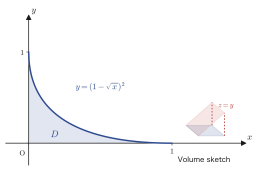
Method 1 (integrate with respect to $y$ first)

$$ V=\int_0^1\int_0^{(1-\sqrt{x})^2} y\,dy\,dx $$

For the inner integral, since an antiderivative of $y$ is $y^2/2$, we have

$$ \int_0^{(1-\sqrt{x})^2} y\,dy=\Big[\frac{y^2}{2}\Big]_0^{(1-\sqrt{x})^2}=\frac{1}{2}(1-\sqrt{x})^4 $$

Therefore it suffices to compute

$$ V=\int_0^1 \frac{1}{2}(1-\sqrt{x})^4\,dx $$

Using the substitution $t=1-\sqrt{x}$ (so $x=(1-t)^2$, $dx=-2(1-t)\,dt$, and $t:1\to0$ when $x:0\to1$), we get

$$ V=\int_1^0 \frac{1}{2}t^4\cdot\{-2(1-t)\}\,dt=\int_0^1 t^4(1-t)\,dt=\int_0^1(t^4-t^5)\,dt=\Big[\frac{t^5}{5}-\frac{t^6}{6}\Big]_0^1=\frac{1}{5}-\frac{1}{6}=\frac{1}{30} $$

(The original notes did not write out the intermediate steps of the substitution and recorded only the result, so here we have supplied the entire computation of the integration by substitution.) Hence $V=\dfrac{1}{30}$.

Method 2 (integrate with respect to $x$ first). This time, solving the boundary equation $y=(1-\sqrt{x})^2$ for $x$, we find by symmetry that $x=(1-\sqrt{y})^2$ ($0\le y\le1$), and

$$ V=\int_0^1\int_0^{(1-\sqrt{y})^2} y\,dx\,dy $$

In the inner integral, the integrand $y$ is a constant that does not depend on $x$, so we only need to multiply by the width in $x$.

$$ \int_0^{(1-\sqrt{y})^2} y\,dx=y\cdot(1-\sqrt{y})^2 $$

Therefore we compute

$$ V=\int_0^1 y(1-\sqrt{y})^2\,dy $$

Expanding $(1-\sqrt{y})^2=1-2\sqrt{y}+y$, we get

$$ V=\int_0^1\left(y-2y^{3/2}+y^2\right)dy=\Big[\frac{y^2}{2}-2\cdot\frac{y^{5/2}}{5/2}+\frac{y^3}{3}\Big]_0^1=\frac12-\frac45+\frac13 $$

Putting the fractions over a common denominator gives $\dfrac12-\dfrac45+\dfrac13=\dfrac{15}{30}-\dfrac{24}{30}+\dfrac{10}{30}=\dfrac{1}{30}$. This agrees with Method 1 (both methods verified with SymPy; the original notes also record the same result $\frac{1}{30}$).

Example 7.3: An improper multiple integral whose integrand diverges at the origin

Find the improper multiple integral $\displaystyle\iint_D\frac{dxdy}{\sqrt{x^2+y^2}}$ of the function $f(x,y)=\dfrac{1}{\sqrt{x^2+y^2}}$ over the region $D=\{(x,y)\mid 0\le y\le x\le1\}$ (a right triangle with a vertex at the origin $(0,0)$).

Solution. The integrand $f(x,y)=1/\sqrt{x^2+y^2}$ diverges at the origin $(0,0)$, where the denominator becomes $0$. In $D$, the origin falls exactly on a vertex of the triangle. Figure 7.5 shows this divergence as a three-dimensional picture (as we approach the origin, the surface $z=f(x,y)$ stretches without bound both upward and downward, taking the shape of a funnel (horn)). We therefore first consider only the part $x\ge c$ ($c$ a small positive number), and let $c\to+0$ afterwards.

$$ V=\iint_D \frac{dxdy}{\sqrt{x^2+y^2}}=\lim_{c\to+0}\int_c^1\int_0^{x}\frac{1}{\sqrt{x^2+y^2}}\,dy\,dx $$

Setting $a=x$ in this formula (we integrate with respect to $y$ treating $x$ as a constant, so $a^2=x^2$), the inner integral is

$$ \int_0^{x}\frac{1}{\sqrt{x^2+y^2}}\,dy=\Big[\ln\big|y+\sqrt{x^2+y^2}\big|\Big]_0^{x} =\ln\big|x+\sqrt{2}\,x\big|-\ln|x| $$

(Substituting $y=x$ gives $\sqrt{x^2+x^2}=\sqrt{2x^2}=\sqrt2\,x$ (since $x>0$), and substituting $y=0$ gives $\sqrt{x^2}=x$.) Using the property of logarithms $\ln A-\ln B=\ln(A/B)$ to simplify, we get

$$ \ln\big|(1+\sqrt2)x\big|-\ln|x|=\ln(1+\sqrt2)+\ln x-\ln x=\ln(1+\sqrt2) $$

This is a constant that does not depend on $x$ at all (this reflects the fact that the integrand $1/\sqrt{x^2+y^2}$ has the property—homogeneity—that “its value does not change when $x,y$ are enlarged or reduced by the same factor”). Therefore,

$$ V=\lim_{c\to+0}\int_c^1 \ln(1+\sqrt{2})\,dx=\lim_{c\to+0}\Big\{(1-c)\ln(1+\sqrt2)\Big\}=\ln(1+\sqrt2) $$

(Since $\ln(1+\sqrt2)$ is a constant independent of $x$, integrating with respect to $x$ merely multiplies it by the width $(1-c)$.) As $c\to+0$ we have $1-c\to1$, so finally we obtain

$$ \iint_D\frac{dxdy}{\sqrt{x^2+y^2}}=\ln(1+\sqrt2)\approx0.8814 $$

(verified with SymPy).

Example 7.4: An improper multiple integral over an unbounded region

Find the improper multiple integral $\displaystyle\iint_D\frac{dxdy}{x^4+y^2}$ of the function $f(x,y)=\dfrac{1}{x^4+y^2}$ over the region $D=\{(x,y)\mid 1\le x,\ 0\le y\le x^2\}$ (a region extending infinitely in the $x$ direction).

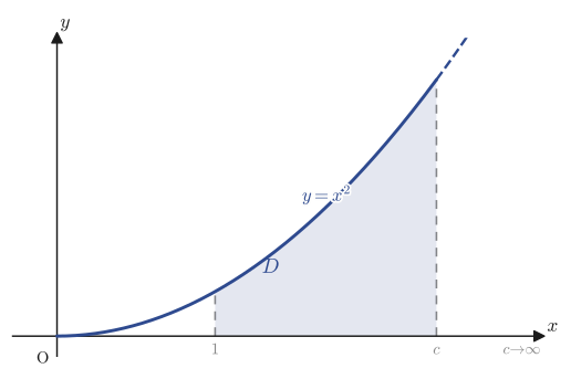
Solution. Since the region extends all the way to $x\to\infty$, we cut it off at $1\le x\le c$ ($c$ is a large positive number), compute, and let $c\to\infty$ afterward.

$$ V=\iint_D\frac{dxdy}{x^4+y^2}=\lim_{c\to\infty}\int_1^c\int_0^{x^2}\frac{1}{x^4+y^2}\,dy\,dx $$

In the inner integral we regard $x$ as a constant. Noting that we can factor $x^4+y^2=x^4\left(1+\left(\dfrac{y}{x^2}\right)^2\right)$, we can use the integration formula for the inverse tangent function, $\displaystyle\int\frac{dt}{1+t^2}=\tan^{-1}t+C$ ($t=y/x^2$, $dt=dy/x^2$).

$$ \int_0^{x^2}\frac{1}{x^4+y^2}\,dy=\frac{1}{x^4}\int_0^{x^2}\frac{1}{1+\left(\frac{y}{x^2}\right)^2}\,dy =\frac{1}{x^4}\left[x^2\tan^{-1}\frac{y}{x^2}\right]_0^{x^2} $$

(Substituting $t=y/x^2$ gives $dy=x^2\,dt$, so $\displaystyle\int\frac{dy}{1+(y/x^2)^2}=x^2\int\frac{dt}{1+t^2}=x^2\tan^{-1}t=x^2\tan^{-1}(y/x^2)$.) Substituting $y=x^2$ gives $\tan^{-1}(x^2/x^2)=\tan^{-1}1=\dfrac{\pi}{4}$, and substituting $y=0$ gives $\tan^{-1}0=0$. Therefore we obtain

$$ \int_0^{x^2}\frac{1}{x^4+y^2}\,dy=\frac{1}{x^4}\cdot x^2\left(\frac{\pi}{4}-0\right)=\frac{1}{x^2}\cdot\frac{\pi}{4} $$

Integrating this from $x=1$ to $x=c$, we get

$$ V=\lim_{c\to\infty}\int_1^c \frac{\pi}{4}\cdot\frac{1}{x^2}\,dx =\lim_{c\to\infty}\frac{\pi}{4}\left[-\frac{1}{x}\right]_1^{c} =\lim_{c\to\infty}\frac{\pi}{4}\left(1-\frac{1}{c}\right) $$

Since $1/c\to0$ as $c\to\infty$, we obtain

$$ \iint_D\frac{dxdy}{x^4+y^2}=\frac{\pi}{4} $$

(Verified with SymPy. In the computation in the original notes, there was a small note in the margin confirming the intermediate evaluations $\tan^{-1}1=\pi/4$ and $\tan^{-1}0=0$, so the main text also states the basis for those evaluations explicitly.)

Example 7.5: The Jacobian and the multiple integral for the change of variables $2x+y=u,\ 2x-y=v$

Solve the question posed at the beginning of this section ($D=\{0\le2x+y\le\pi,\ 0\le2x-y\le\pi\}$, $f(x,y)=(2x+y)\sin(2x-y)$) by actually carrying out a change of variables.

Solution. Since $x=\dfrac{u+v}{4}$ and $y=\dfrac{u-v}{2}$, the Jacobian matrix is

$$ J=\begin{pmatrix}\pdiff{x}{u}&\pdiff{x}{v}\\[2mm]\pdiff{y}{u}&\pdiff{y}{v}\end{pmatrix}=\begin{pmatrix}\dfrac14&\dfrac14\\[2mm]\dfrac12&-\dfrac12\end{pmatrix} $$

(Differentiating $x=(u+v)/4$ partially with respect to $u$ gives $1/4$, and differentiating with respect to $v$ also gives $1/4$. Differentiating $y=(u-v)/2$ partially with respect to $u$ gives $1/2$, and differentiating with respect to $v$ gives $-1/2$.) Using the formula for a determinant of order 2 in Definition 7.2 (see the Math Note), the Jacobian is

$$ \det J=\frac14\times\left(-\frac12\right)-\frac14\times\frac12=-\frac18-\frac18=-\frac14,\qquad |J|=\frac14 $$

Therefore $dxdy=\dfrac14\,dudv$. Directly from the definitions $u=2x+y$ and $v=2x-y$, the region $D$ corresponds to $0\le u\le\pi$, $0\le v\le\pi$ (a square of side $\pi$). The multiple integral can be rewritten as

$$ \iint_D(2x+y)\sin(2x-y)\,dxdy=\int_0^\pi\int_0^\pi u\sin v\cdot\frac14\,dudv $$

Since the integrand is the product of a function of $u$ alone and a function of $v$ alone, it can be factored into a product of two single-variable integrals (we will use this technique repeatedly from the next section on). Thus we obtain

$$ =\frac14\left(\int_0^\pi u\,du\right)\left(\int_0^\pi\sin v\,dv\right) =\frac14\cdot\Big[\frac{u^2}{2}\Big]_0^\pi\cdot\Big[-\cos v\Big]_0^\pi =\frac14\cdot\frac{\pi^2}{2}\cdot\big(-(-1)-(-1)\big) $$

(Here $\big[-\cos v\big]_0^\pi=-\cos\pi-(-\cos0)=-(-1)-(-1)=1+1=2$.)

$$ =\frac14\cdot\frac{\pi^2}{2}\cdot2=\frac{\pi^2}{4} $$

In this way, we have seen that the multiple integral, which at first looked hard to compute, can be solved in just a few lines by the change of coordinates using the Jacobian (verified with SymPy). Incidentally, this pair $u=2x+y,\,v=2x-y$ is an example of a pair of coordinate axes that are not mutually orthogonal—oblique coordinates (the line along which the value of $u$ is constant, $2x+y=$ (constant), and the line along which the value of $v$ is constant, $2x-y=$ (constant), do not meet at right angles).

Example 7.6: Change of variables on a parallelogram region

Find the multiple integral $V=\displaystyle\iint_D f(x,y)\,dxdy$ of the function $f(x,y)=\dfrac{\tan^{-1}(x-y)}{x+y}$ over the region $D=\left\{(x,y)\;\middle|\; 1\le x+y\le 2,\ 0\le x-y\le 1\right\}$ (a parallelogram).

Solution. Let $u=x+y$ and $v=x-y$; then $D$ corresponds to $1\le u\le2$, $0\le v\le1$ (a rectangle). To find the Jacobian, we may express $x,y$ in terms of $u,v$ and compute directly, or we may use the shortcut described in the Caution (Section 7.3, Eq. \eqref{eq:7-inverse-jacobian})—first computing the Jacobian matrix $J_2$ of the inverse transformation $u=u(x,y),v=v(x,y)$, and then setting $|\det J_1|=1/|\det J_2|$. Here we use the shortcut. Partially differentiating $u=x+y,\,v=x-y$ with respect to $x,y$, we obtain

$$ J_2=\begin{pmatrix}\pdiff{u}{x}&\pdiff{u}{y}\\[2mm]\pdiff{v}{x}&\pdiff{v}{y}\end{pmatrix}=\begin{pmatrix}1&1\\1&-1\end{pmatrix},\qquad \det J_2=1\times(-1)-1\times1=-2 $$

Therefore $|\det J_1|=1/|\det J_2|=1/2$. (If we compute $J_1$ directly from $x=(u+v)/2$ and $y=(u-v)/2$, then $\det J_1=\dfrac12\times\left(-\dfrac12\right)-\dfrac12\times\dfrac12=-\dfrac14-\dfrac14=-\dfrac12$, so $|\det J_1|=1/2$, which agrees. The computation in the original notes was written as a mixture of these two ways of computing—the relation $1/|\det J_2|$ coming from the inverse matrix and the directly computed $|\det J_1|$—so this book presents the two justifications separately.) Hence $dxdy=\dfrac12\,dudv$. The integrand can be rewritten as $f=\dfrac{\tan^{-1}(x-y)}{x+y}=\dfrac{\tan^{-1}v}{u}$, so

$$ V=\int_0^1\int_1^2 \frac{\tan^{-1}v}{u}\cdot\frac12\,dudv =\frac12\left(\int_1^2\frac{du}{u}\right)\left(\int_0^1\tan^{-1}v\,dv\right) $$

(Since the integrand is the product of a function of $u$ alone and a function of $v$ alone, the integral can be factored into a product of two single-variable integrals regardless of the order of integration.) First, the integral in $u$ is

$$ \int_1^2\frac{du}{u}=\big[\ln u\big]_1^2=\ln2-\ln1=\ln2 $$

Next, for the integral in $v$, $\displaystyle\int_0^1\tan^{-1}v\,dv$, we use integration by parts. Let $f=\tan^{-1}v$ and $dg=dv$; then $df=\dfrac{dv}{1+v^2}$ and $g=v$, so

$$ \int\tan^{-1}v\,dv=v\tan^{-1}v-\int\frac{v}{1+v^2}\,dv=v\tan^{-1}v-\frac12\ln(1+v^2)+C $$

(For $\displaystyle\int\frac{v}{1+v^2}dv$, the numerator is half the derivative of the denominator $\left(\frac{d}{dv}(1+v^2)=2v\right)$, so the substitution $t=1+v^2$ gives $\frac12\ln|t|=\frac12\ln(1+v^2)$.) Therefore we obtain

$$ \int_0^1\tan^{-1}v\,dv=\Big[v\tan^{-1}v-\frac12\ln(1+v^2)\Big]_0^1 =\left(1\cdot\frac{\pi}{4}-\frac12\ln2\right)-(0-0)=\frac{\pi}{4}-\frac12\ln2 $$

Putting everything together, we obtain

$$ V=\frac12\cdot\ln2\cdot\left(\frac{\pi}{4}-\frac12\ln2\right)=\frac{\ln2}{2}\left(\frac{\pi}{4}-\frac{\ln2}{2}\right)=\frac{1}{8}(\pi-2\ln2)\ln2 $$

(verified with SymPy; numerically, $V\approx0.1521$).

Example 7.7: Volume of the intersection of a hemisphere and a cylinder

Find the volume $V$ of the intersection of the hemisphere $x^2+y^2+z^2\le4,\ z\ge0$ and the cylinder $(x-1)^2+y^2\le1$.

Solution. The equation of the hemisphere is $z=\sqrt{4-(x^2+y^2)}$ (obtained by solving $x^2+y^2+z^2=4$ for $z$ in the range $z\ge0$). Therefore the required volume is the integral of the height of the hemisphere over the base $D=\{(x,y)\mid(x-1)^2+y^2\le1\}$ of the cylinder, namely

$$ V=\iint_D\sqrt{4-(x^2+y^2)}\,dxdy $$

Using polar coordinates $x=r\cos\theta,\,y=r\sin\theta$ (with Jacobian $|J|=r$, Eq. \eqref{eq:7-polar-jacobian}; we derive it again in Example 7.8 of Section 7.5), the expression for the boundary of the cylinder becomes

$$ (r\cos\theta-1)^2+(r\sin\theta)^2\le1 \ \Longrightarrow\ r^2\cos^2\theta-2r\cos\theta+1+r^2\sin^2\theta\le1 \ \Longrightarrow\ r^2-2r\cos\theta\le0 $$

(We simplified using $\cos^2\theta+\sin^2\theta=1$.) This factors as $r(r-2\cos\theta)\le0$, and since $r\ge0$, it means $0\le r\le2\cos\theta$ (this is meaningful only in the range $-\dfrac{\pi}{2}\le\theta\le\dfrac{\pi}{2}$, where $\cos\theta\ge0$; it is the circle with center $(1,0)$ and radius $1$ (the circle through the origin, $(x-1)^2+y^2=1$), and it is the region shown on the right of Figure 7.9). Hence,

$$ V=\iint_{D'}\sqrt{4-r^2}\cdot r\,drd\theta,\qquad D'=\left\{0\le r\le2\cos\theta,\ -\frac{\pi}{2}\le\theta\le\frac{\pi}{2}\right\} $$

Here, both the integrand and the region of integration are invariant under the transformation $\theta\to-\theta$ (since $\cos(-\theta)=\cos\theta$, the upper limit $2\cos\theta$ does not change either). Therefore it suffices to halve the interval of integration for $\theta$ to $[0,\pi/2]$ and double the result.

$$ V=2\int_0^{\pi/2}\int_0^{2\cos\theta}\sqrt{4-r^2}\,r\,drd\theta $$

For the inner integral, substituting $w=4-r^2$ ($dw=-2r\,dr$) gives

$$ \int r\sqrt{4-r^2}\,dr=-\frac12\int\sqrt{w}\,dw=-\frac12\cdot\frac{2}{3}w^{3/2}=-\frac13(4-r^2)^{3/2}+C $$

Therefore,

$$ \int_0^{2\cos\theta}\sqrt{4-r^2}\,r\,dr=\Big[-\frac13(4-r^2)^{3/2}\Big]_0^{2\cos\theta} =-\frac13(4-4\cos^2\theta)^{3/2}+\frac13\cdot4^{3/2} $$

We have $4-4\cos^2\theta=4\sin^2\theta$, and since $\sin\theta\ge0$ for $0\le\theta\le\pi/2$, $(4\sin^2\theta)^{3/2}=8\sin^3\theta$. Also, $4^{3/2}=8$. Hence we obtain

$$ \int_0^{2\cos\theta}\sqrt{4-r^2}\,r\,dr=-\frac83\sin^3\theta+\frac83=\frac83\left(1-\sin^3\theta\right) $$

Integrating this with respect to $\theta$, we get

$$ V=2\int_0^{\pi/2}\frac83\left(1-\sin^3\theta\right)d\theta=\frac{16}{3}\left(\int_0^{\pi/2}d\theta-\int_0^{\pi/2}\sin^3\theta\,d\theta\right) $$

We have $\displaystyle\int_0^{\pi/2}d\theta=\dfrac{\pi}{2}$. To evaluate $\displaystyle\int_0^{\pi/2}\sin^3\theta\,d\theta$, we decompose $\sin^3\theta=\sin\theta(1-\cos^2\theta)=\sin\theta-\sin\theta\cos^2\theta$ and substitute $c=\cos\theta$ ($dc=-\sin\theta\,d\theta$), which gives

$$ \int_0^{\pi/2}\sin^3\theta\,d\theta=\int_1^0(1-c^2)(-dc)=\int_0^1(1-c^2)\,dc=\Big[c-\frac{c^3}{3}\Big]_0^1=1-\frac13=\frac23 $$

Therefore we obtain

$$ V=\frac{16}{3}\left(\frac{\pi}{2}-\frac23\right)=\frac{16}{3}\cdot\frac{\pi}{2}-\frac{16}{3}\cdot\frac23=\frac{8\pi}{3}-\frac{32}{9}=\frac{24\pi-32}{9}=\frac89(3\pi-4) $$

(verified with SymPy; numerically, $V\approx4.822$).

Example 7.8: Proof of the Gaussian integral (the method using polar coordinates)

By converting the double integral $\displaystyle\int_{-\infty}^{\infty}\int_{-\infty}^{\infty} e^{-x^2-y^2}\,dxdy$ to polar coordinates and evaluating it, prove that $\displaystyle\int_{-\infty}^{\infty}e^{-x^2}\,dx=\sqrt{\pi}$.

Solution. First, we confirm the relation between the double integral and the single-variable integral. The integration variables $x,y$ each range independently from $-\infty$ to $\infty$, so, using the law of exponents $e^{-x^2-y^2}=e^{-x^2}\cdot e^{-y^2}$, the double integral splits into a product of two identical single-variable integrals.

$$ \int_{-\infty}^{\infty}\int_{-\infty}^{\infty} e^{-x^2-y^2}\,dxdy =\left(\int_{-\infty}^{\infty}e^{-x^2}dx\right)\left(\int_{-\infty}^{\infty}e^{-y^2}dy\right) =\left(\int_{-\infty}^{\infty}e^{-x^2}dx\right)^2 $$

(The integral with respect to $x$ and the integral with respect to $y$ have the same value; only the names of the variables differ.) Therefore, once the value of this double integral is found, its square root is the value of the Gaussian integral. So we change to the polar coordinates $x=r\cos\theta,\ y=r\sin\theta$ ($0\le r\lt\infty,\ 0\le\theta\lt2\pi$, which cover the entire plane). We have $x^2+y^2=r^2\cos^2\theta+r^2\sin^2\theta=r^2$, and, following Definition 7.2, the Jacobian is

\begin{equation} |J|=\left|\begin{vmatrix} \pdiff{x}{r} & \pdiff{x}{\theta} \\[2mm] \pdiff{y}{r} & \pdiff{y}{\theta} \end{vmatrix}\right| =\left|\begin{vmatrix} \cos\theta & -r\sin\theta \\ \sin\theta & r\cos\theta \end{vmatrix}\right| =\big|r\cos^2\theta-(-r\sin\theta)\sin\theta\big|=\big|r(\cos^2\theta+\sin^2\theta)\big|=r \label{eq:7-polar-jacobian} \end{equation}

(Since $r\ge0$, the absolute value can be dropped.) This is the Jacobian of the polar coordinate transformation, and we have $dxdy=r\,drd\theta$. Therefore,

$$ \int_{-\infty}^{\infty}\int_{-\infty}^{\infty} e^{-x^2-y^2}\,dxdy = \int_0^{2\pi}\int_0^{\infty} e^{-r^2}\,r\,drd\theta $$

The integrand $e^{-r^2}r$ is treated as an improper integral over the unbounded interval $[0,\infty)$. Taking the limit $c\to\infty$ and using the substitution $w=-r^2$ ($dw=-2r\,dr$), we get

$$ \int_0^{\infty} e^{-r^2}\,r\,dr=\lim_{c\to\infty}\int_0^{c}e^{-r^2}r\,dr=\lim_{c\to\infty}\Big[-\frac12e^{-r^2}\Big]_0^{c} =\lim_{c\to\infty}\left(-\frac12e^{-c^2}+\frac12\right)=\frac12 $$

(Since $e^{-c^2}\to0$ as $c\to\infty$, the first term vanishes.) The result $1/2$ of the $r$-integral is a constant that does not depend on $\theta$, so we obtain

$$ \int_0^{2\pi}\int_0^{\infty} e^{-r^2}\,r\,drd\theta=\int_0^{2\pi}\frac12\,d\theta=\frac12\cdot2\pi=\pi $$

That is, $\left(\displaystyle\int_{-\infty}^{\infty}e^{-x^2}dx\right)^2=\pi$. Since $e^{-x^2}\gt0$, the integral itself is positive, so, taking the square root, we obtain

$$ \int_{-\infty}^{\infty}e^{-x^2}\,dx=\sqrt{\pi} $$

(verified with SymPy).

Example 7.9: Alternative proof of the Gaussian integral (the squeeze theorem)

For $R\gt0$, consider the following three regions in the first quadrant:

$$ B_R=\left\{(x,y)\;\middle|\;x^2+y^2\le R^2,\,x\ge0,\,y\ge0\right\},\qquad A_R=\{(x,y)\mid0\le x\le R,\,0\le y\le R\},\qquad B_{\sqrt2R}=\left\{(x,y)\;\middle|\;x^2+y^2\le2R^2,\,x\ge0,\,y\ge0\right\} $$

($B_R$ is the quarter disk of radius $R$, $A_R$ is the square of side $R$, and $B_{\sqrt2R}$ is the quarter disk of radius $\sqrt2R$.) Using the fact that $B_R\subset A_R\subset B_{\sqrt2R}$ (Figure 7.10), show that $\displaystyle\int_0^{\infty}e^{-x^2}\,dx=\dfrac{\sqrt\pi}{2}$.

Solution. Since $f(x,y)=e^{-x^2-y^2}\ge0$, the larger the region, the larger the value of the double integral (enlarging the region only adds nonnegative quantities). Therefore, from $B_R\subset A_R\subset B_{\sqrt2R}$ we immediately obtain the inequality

$$ \iint_{B_R}e^{-x^2-y^2}dxdy\ \le\ \iint_{A_R}e^{-x^2-y^2}dxdy\ \le\ \iint_{B_{\sqrt2R}}e^{-x^2-y^2}dxdy $$

(In the notation of the original notes, this inequality reads $I_R\le J_R\le I_{\sqrt2R}$.) Let us compute each of the three double integrals. The double integral $J_R$ over the square $A_R$ can be evaluated directly as an iterated integral, since the region is a rectangle, and the same decomposition by the law of exponents as in Example 7.8 can be used.

$$ J_R=\int_0^R\int_0^R e^{-x^2}\cdot e^{-y^2}\,dxdy=\left(\int_0^R e^{-x^2}dx\right)\left(\int_0^R e^{-y^2}dy\right)=\left(\int_0^R e^{-x^2}dx\right)^2 $$

For the double integral $I_R$ over the sector $B_R$, it suffices to convert to polar coordinates ($0\le r\le R,\ 0\le\theta\le\pi/2$). Carrying out the same computation as in Example 7.8, but cutting off the upper limit of integration at $R$ instead of $\infty$, we get

$$ I_R=\int_0^{\pi/2}\int_0^R e^{-r^2}\cdot r\,drd\theta =\int_0^{\pi/2}\Big[-\frac12e^{-r^2}\Big]_0^Rd\theta =\int_0^{\pi/2}\frac12\left(1-e^{-R^2}\right)d\theta =\frac{\pi}{4}\left(1-e^{-R^2}\right) $$

Similarly, for $B_{\sqrt2R}$ we only replace the radius by $\sqrt2R$, so we obtain

$$ I_{\sqrt2R}=\int_0^{\pi/2}\int_0^{\sqrt2R} e^{-r^2}\cdot r\,drd\theta=\frac{\pi}{4}\left(1-e^{-2R^2}\right) $$

Substituting the above into the squeeze inequality, we get

$$ \frac{\pi}{4}\left(1-e^{-R^2}\right)\ \le\ \left(\int_0^R e^{-x^2}dx\right)^2\ \le\ \frac{\pi}{4}\left(1-e^{-2R^2}\right) $$

As $R\to\infty$, we have $e^{-R^2}\to0$ and $e^{-2R^2}\to0$, so both the left and right ends converge to $\dfrac{\pi}{4}$. By the squeeze theorem (if the left and right sides converge to the same value, the quantity between them also converges to that value), we obtain

$$ \lim_{R\to\infty}\left(\int_0^R e^{-x^2}dx\right)^2=\frac{\pi}{4} $$

The left-hand side equals $\displaystyle\left(\int_0^{\infty}e^{-x^2}dx\right)^2$ (this is exactly the definition of the improper integral), so, taking the square root of both sides (the integral is positive since $e^{-x^2}\gt0$), we obtain

$$ \int_0^{\infty}e^{-x^2}\,dx=\sqrt{\frac{\pi}{4}}=\frac{\sqrt\pi}{2} $$

(verified with SymPy. It is also consistent with the fact that the result $\displaystyle\int_{-\infty}^{\infty}e^{-x^2}dx=\sqrt\pi$ of Example 7.8, together with the evenness of $e^{-x^2}$, gives $\displaystyle\int_0^{\infty}e^{-x^2}dx=\frac12\int_{-\infty}^{\infty}e^{-x^2}dx=\frac{\sqrt\pi}{2}$.)

Example 7.10: A change of variables that rotates a rhombic region by 45 degrees

Find the double integral $V=\displaystyle\iint_D f(x,y)\,dxdy$ of the function $f(x,y)=(x+y)e^{x-y}$ over the region $D=\{(x,y)\mid|x-1|+|y|\le1\}$ (Figure 7.11, left; a rhombus with center $(1,0)$ and vertices $(0,0),(1,1),(2,0),(1,-1)$).

Solution. We define the new variables by $u=\dfrac{x+y}{\sqrt2}$ and $v=\dfrac{x-y}{\sqrt2}$ (this transformation rotates the coordinate axes about the origin by $-45°$). Solving these equations in the reverse direction gives

$$ x=\frac{u+v}{\sqrt2},\qquad y=\frac{u-v}{\sqrt2} $$

(adding and subtracting the defining equations side by side confirms that $u+v=\sqrt2 x$ and $u-v=\sqrt2 y$). The Jacobian is

$$ J=\begin{pmatrix}\pdiff{x}{u}&\pdiff{x}{v}\\[2mm]\pdiff{y}{u}&\pdiff{y}{v}\end{pmatrix}=\begin{pmatrix}\dfrac{1}{\sqrt2}&\dfrac{1}{\sqrt2}\\[2mm]\dfrac{1}{\sqrt2}&-\dfrac{1}{\sqrt2}\end{pmatrix},\qquad \det J=\frac{1}{\sqrt2}\times\left(-\frac1{\sqrt2}\right)-\frac1{\sqrt2}\times\frac1{\sqrt2}=-\frac12-\frac12=-1 $$

so $|J|=1$.

Next we check how the region $D$ (the rhombus) is described in terms of $u,v$. Transforming the vertices $(0,0),(1,1),(2,0),(1,-1)$ by $u=(x+y)/\sqrt2,\,v=(x-y)/\sqrt2$, we get, in order, $(0,0)$, $(\sqrt2,0)$, $(\sqrt2,\sqrt2)$, $(0,\sqrt2)$ (for example, for $(1,1)$ we have $u=(1+1)/\sqrt2=\sqrt2,\,v=(1-1)/\sqrt2=0$), and these are nothing other than the four vertices of the square $D'=\{0\le u\le\sqrt2,\,0\le v\le\sqrt2\}$ of side $\sqrt2$. Therefore $D$ is mapped onto $D'$. Finally, we express the integrand in terms of $u,v$. From the definition of $u,v$ we can read off directly that $x+y=\sqrt2\,u$ and $x-y=\sqrt2\,v$ (this is precisely the reason for introducing $u,v$). Hence the integrand becomes

$$ (x+y)e^{x-y}=\sqrt2\,u\cdot e^{\sqrt2\,v} $$

Putting all of this together,

$$ V=\int_0^{\sqrt2}\int_0^{\sqrt2}\sqrt2\,u\,e^{\sqrt2\,v}\,dudv =\sqrt2\left(\int_0^{\sqrt2}u\,du\right)\left(\int_0^{\sqrt2}e^{\sqrt2v}\,dv\right) $$

We have $\displaystyle\int_0^{\sqrt2}u\,du=\Big[\frac{u^2}{2}\Big]_0^{\sqrt2}=\frac{2}{2}=1$ and $\displaystyle\int_0^{\sqrt2}e^{\sqrt2v}\,dv=\frac{1}{\sqrt2}\Big[e^{\sqrt2v}\Big]_0^{\sqrt2}=\frac{1}{\sqrt2}(e^{2}-1)$ (the exponent is $\sqrt2\times\sqrt2=2$). Therefore,

$$ V=\sqrt2\times1\times\frac{1}{\sqrt2}(e^2-1)=e^2-1 $$

is obtained (verified with SymPy; numerically, $V\approx6.389$).

Example 7.11: Volume of a tetrahedron (triple integral)

Find the triple integral $\displaystyle\iiint_V x\,dxdydz$ over the region $V=\{(x,y,z)\mid x,y,z\ge0,\ x+y+z\le1\}$ (the tetrahedron whose vertices are the origin and the three points $(1,0,0),(0,1,0),(0,0,1)$) by two methods that differ in the order of integration.

Solution (Method 1: in the order $z\to y\to x$). First we find the range over which $z$ varies when $x,y$ are fixed. From the conditions $x+y+z\le1,\,z\ge0$ we have

$$ 0\le z\le1-x-y $$

So, if we integrate first with respect to $z$ (the multiple integral of $x$ takes a form in which a multiple integral over the base $D=\{(x,y)\mid x\ge0,y\ge0,x+y\le1\}$ (Figure 7.12, right) still remains), we get

$$ \iiint_V x\,dxdydz=\iint_D\left(\int_0^{1-x-y}x\,dz\right)dxdy=\iint_D x(1-x-y)\,dxdy $$

(The inner integral is just an integration with respect to $z$ with $x$ regarded as a constant, so it becomes $x\cdot(1-x-y)$: we have simply multiplied by the height $1-x-y$.) Next, over $D=\{0\le x\le1,\,0\le y\le1-x\}$, we use the iterated integral that integrates first with respect to $y$ (Formula 7.1 (I)):

$$ =\int_0^1\left\{\int_0^{1-x}(1-x-y)x\,dy\right\}dx $$

The inner integral (integrating with respect to $y$ with $x$ regarded as a constant) is

$$ \int_0^{1-x}(1-x-y)x\,dy=x\Big[(1-x)y-\frac{y^2}{2}\Big]_0^{1-x}=x\left\{(1-x)^2-\frac{(1-x)^2}{2}\right\}=x\cdot\frac{(1-x)^2}{2} $$

(Substituting $y=1-x$ into $(1-x)y$ gives $(1-x)^2$, substituting $y=1-x$ into $y^2/2$ gives $(1-x)^2/2$, and subtracting leaves just half.) Therefore,

$$ \iiint_V x\,dxdydz=\int_0^1\left\{(1-x)^2x-\frac{x}{2}(1-x)^2\right\}dx=\int_0^1\frac{x}{2}(1-x)^2\,dx $$

and it suffices to compute this last integral. Expanding $(1-x)^2=1-2x+x^2$ and simplifying, we get

$$ \frac{x}{2}(1-2x+x^2)=\frac{x}{2}-x^2+\frac{x^3}{2} $$ $$ \int_0^1\left(\frac{x}{2}-x^2+\frac{x^3}{2}\right)dx=\Big[\frac{x^2}{4}-\frac{x^3}{3}+\frac{x^4}{8}\Big]_0^1=\frac14-\frac13+\frac18 $$

Bringing these to a common denominator (24), $\dfrac14-\dfrac13+\dfrac18=\dfrac{6}{24}-\dfrac{8}{24}+\dfrac{3}{24}=\dfrac{1}{24}$. Hence,

$$ \iiint_V x\,dxdydz=\frac{1}{24} $$

is obtained.

Solution (Method 2: in the order $x\to y\to z$, leaving $z$ until the end). This time we first fix $z$, evaluate the double integral with respect to $x,y$ over the horizontal cross section $D_z=\{(x,y)\mid x\ge0,y\ge0,x+y\le1-z\}$ at height $z$ (Figure 7.13; a right triangle whose legs have length $1-z$), and finally integrate with respect to $z$.

$$ \iiint_V x\,dxdydz=\int_0^1\left(\int_0^{1-z}\int_0^{1-z-x}x\,dy\,dx\right)dz $$

The innermost integral (integrating with respect to $y$ with $x,z$ fixed) is, since the integrand $x$ does not depend on $y$,

$$ \int_0^{1-z-x}x\,dy=x(1-z-x) $$

Next we integrate with respect to $x$ from $0$ to $1-z$ ($z$ is again treated as a constant here).

$$ \int_0^{1-z}x(1-z-x)\,dx=\int_0^{1-z}\left\{(1-z)x-x^2\right\}dx =\Big[(1-z)\frac{x^2}{2}-\frac{x^3}{3}\Big]_0^{1-z} $$

Substituting $x=1-z$ gives

$$ (1-z)\cdot\frac{(1-z)^2}{2}-\frac{(1-z)^3}{3}=\frac{(1-z)^3}{2}-\frac{(1-z)^3}{3}=(1-z)^3\left(\frac12-\frac13\right)=\frac{(1-z)^3}{6} $$

(in the original notes this computation was written all at once, in a single line, as $\dfrac16(1-z)^3$, so in this book we have supplied the intermediate step of bringing the fractions to a common denominator). Finally, integrating with respect to $z$,

$$ \iiint_V x\,dxdydz=\int_0^1\frac{(1-z)^3}{6}\,dz=\frac16\Big[-\frac{(1-z)^4}{4}\Big]_0^1=\frac16\left(0+\frac14\right)=\frac{1}{24} $$

is obtained. Both Method 1 and Method 2 gave the same value $\dfrac{1}{24}$ (both methods verified with SymPy).

Example 7.12: Volume of a sphere (three methods)

Find the volume of the sphere $D_1=\{(x,y,z)\mid x^2+y^2+z^2\le R^2\}$ of radius $R$ in three ways.

Method 1 (using the Jacobian of spherical coordinates directly). In spherical coordinates, the sphere $D_1$ is simply described by $0\le r\le R,\ 0\le\theta\le\pi,\ 0\le\varphi\lt2\pi$ ($r$ is the distance from the origin, so it is at most $R$, while $\theta,\varphi$ range over all directions without restriction). Using the Jacobian we derived earlier (Eq. \eqref{eq:7-spherical-jacobian}), we have

$$ \iiint_{D_1}dxdydz=\int_0^{2\pi}\int_0^{\pi}\int_0^R r^2\sin\theta\,drd\theta d\varphi $$

Since the integrand factors into a product of functions each depending on only one of $r,\theta,\varphi$, the integral becomes a product of three single-variable integrals.

$$ =\left(\int_0^R r^2\,dr\right)\left(\int_0^{\pi}\sin\theta\,d\theta\right)\left(\int_0^{2\pi}d\varphi\right) =\Big[\frac{r^3}{3}\Big]_0^R\cdot\Big[-\cos\theta\Big]_0^{\pi}\cdot\big[\varphi\big]_0^{2\pi} $$ $$ =\frac{R^3}{3}\times\big(-\cos\pi-(-\cos0)\big)\times2\pi=\frac{R^3}{3}\times\big(1+1\big)\times2\pi=\frac{R^3}{3}\times2\times2\pi=\frac{4}{3}\pi R^3 $$

This gives the result.

Method 2 (polar coordinates + cross-section integral for the hemisphere). The upper half of the sphere ($z\ge0$) is the surface $z=\sqrt{R^2-x^2-y^2}$, and the volume beneath it is a multiple integral of exactly the same form as in Example 7.7 of Section 7.4. The volume of the whole sphere is twice this, so

$$ V=2\iint_{D_2}\sqrt{R^2-x^2-y^2}\,dxdy,\qquad D_2=\{(x,y)\mid x^2+y^2\le R^2\} $$

($D_2$ is a disk of radius $R$; it corresponds to the equator of the sphere in the $xy$-plane.) Using two-dimensional polar coordinates $x=r\cos\theta,\,y=r\sin\theta$ ($dxdy=rdrd\theta$), we have

$$ V=2\int_0^{2\pi}\int_0^R\sqrt{R^2-r^2}\,r\,drd\theta $$

As in Example 7.7, for the inner integral we use the substitution $w=R^2-r^2$, which gives

$$ \int_0^R r\sqrt{R^2-r^2}\,dr=\Big[-\frac13(R^2-r^2)^{3/2}\Big]_0^R=0-\left(-\frac13R^3\right)=\frac{R^3}{3} $$

Hence

$$ V=2\int_0^{2\pi}\frac{R^3}{3}\,d\theta=2\cdot\frac{R^3}{3}\cdot2\pi=\frac{4}{3}\pi R^3 $$

This gives the result.

Method 3 (a simple cross-section integral, using neither spherical nor polar coordinates). We directly use the formula “volume as the integral of cross-sectional area” that you learned in high school mathematics. If we cut the sphere by the horizontal plane at height $z$ ($-R\le z\le R$), the cross section is a circle of radius $\sqrt{R^2-z^2}$ (Figure 7.15; this can be seen by substituting a fixed value of $z$ into the equation of the sphere $x^2+y^2+z^2=R^2$: on the cross section, $x^2+y^2=R^2-z^2$ is the equation of a circle). The cross-sectional area is $\pi(R^2-z^2)$ (the square of the radius $\times\pi$), so

$$ V=\int_{-R}^R \pi(R^2-z^2)\,dz=\pi\Big[R^2z-\frac{z^3}{3}\Big]_{-R}^R $$ $$ =\pi\left\{\left(R^3-\frac{R^3}{3}\right)-\left(-R^3+\frac{R^3}{3}\right)\right\}=\pi\left(\frac{2R^3}{3}+\frac{2R^3}{3}\right)=\pi\cdot\frac{4R^3}{3}=\frac{4}{3}\pi R^3 $$

This gives the result. All three methods have led to the same answer $\dfrac{4}{3}\pi R^3$, the very formula for the volume of a sphere that you memorized in high school mathematics (verified with SymPy for all three methods). Each method has its strengths and weaknesses. Method 1 (spherical coordinates) is the most mechanical and the easiest to follow, but it requires remembering the Jacobian of spherical coordinates. Method 2 (polar coordinates + cross-section integral) can be computed as an extension of the techniques of the preceding sections. Method 3 is the most elementary, but it requires the geometric insight that “the cross section is a circle” beforehand.

Example 7.13: Surface area of a sphere (two methods)

Find the surface area of the sphere $x^2+y^2+z^2=R^2$ of radius $R$ by two methods.

Method 1 (using the surface area formula). The upper hemisphere is $z=\sqrt{R^2-x^2-y^2}$, and the surface area of the whole sphere is twice the area of the upper hemisphere. Differentiating $x^2+y^2+z^2=R^2$ partially with respect to $x$ and $y$ (we differentiate it as an implicit function; note that $z$ is also a function of $x,y$), we have

$$ 2x+2z\pdiff zx=0,\qquad2y+2z\pdiff zy=0 \ \Longrightarrow\ \pdiff zx=-\frac xz,\qquad\pdiff zy=-\frac yz $$

Therefore,

$$ \left(\pdiff zx\right)^2+\left(\pdiff zy\right)^2+1=\frac{x^2}{z^2}+\frac{y^2}{z^2}+1=\frac{x^2+y^2+z^2}{z^2}=\frac{R^2}{z^2} $$

(In the last step we used the equation of the sphere $x^2+y^2+z^2=R^2$.) Substituting into the surface area formula (Eq. \eqref{eq:7-surface-element}), with $D$ the equatorial disk $\{x^2+y^2\le R^2\}$ of the sphere, we get

$$ S=2\iint_D\sqrt{\frac{R^2}{z^2}}\,dxdy=2\iint_D\frac{R}{\sqrt{R^2-x^2-y^2}}\,dxdy $$

(The factor 2 accounts for the upper and lower hemispheres. We have $\sqrt{R^2/z^2}=R/|z|=R/z$, and since $z\ge0$ the absolute value can be dropped. We also substituted $z=\sqrt{R^2-x^2-y^2}$.) Using polar coordinates $x=r\cos\theta,\,y=r\sin\theta$ ($dxdy=rdrd\theta$), we obtain

$$ S=2\int_0^{2\pi}\int_0^R\frac{R}{\sqrt{R^2-r^2}}\,r\,drd\theta $$

For the inner integral, using the substitution $w=R^2-r^2$ ($dw=-2rdr$), we have

$$ \int_0^R\frac{r}{\sqrt{R^2-r^2}}\,dr=\Big[-\sqrt{R^2-r^2}\Big]_0^R=0-(-R)=R $$

(This is an improper integral and should properly be treated as a limit as $r\to R$, but since the convergence $-\sqrt{R^2-r^2}\to0$ causes no problem, the result does not change.) Therefore,

$$ S=2\int_0^{2\pi}R\cdot R\,d\theta=2R^2\int_0^{2\pi}d\theta=2R^2\cdot2\pi=4\pi R^2 $$

This gives the result.

Method 2 (using the Jacobian of spherical coordinates). Every point on the sphere of radius $R$ is expressed in spherical coordinates by $r=R$ (constant), and $\theta,\varphi$ vary over it. Setting $r=R$ (constant) in the Jacobian we derived earlier (Eq. \eqref{eq:7-spherical-jacobian}), $dxdydz=r^2\sin\theta\,drd\theta d\varphi$, gives the area element on the sphere, $dS=R^2\sin\theta\,d\theta d\varphi$ (since we consider only the sphere of constant radius $R$, we do not integrate in the $dr$ direction, and it suffices to substitute $R^2$ for $r^2$). Therefore,

$$ S=\int_0^{2\pi}\int_0^{\pi}R^2\sin\theta\,d\theta d\varphi=R^2\left(\int_0^{\pi}\sin\theta\,d\theta\right)\left(\int_0^{2\pi}d\varphi\right)=R^2\cdot\big[-\cos\theta\big]_0^{\pi}\cdot2\pi $$ $$ =R^2\times2\times2\pi=4\pi R^2 $$

This gives the result. The two methods agree (verified with SymPy for both methods. The result agrees with the formula $4\pi R^2$ for the surface area of a sphere that you memorized in high school mathematics. Incidentally, differentiating $S=4\pi R^2$ with respect to $R$ gives $dS/dR=8\pi R=2\times4\pi R$, and it is useful to remember that this coincides with $dV/dR=4\pi R^2=S$, obtained by differentiating the volume formula $V=\frac43\pi R^3$ with respect to $R$: this is because the increase in volume when the radius is increased by $dR$ is approximately equal to the volume of a thin skin of thickness $dR$ laid over the entire surface).

Exercise 7.1: Multiple integral over a triangular region

Find the multiple integral $\displaystyle\iint_D(x+y)\,dxdy$ of the function $f(x,y)=x+y$ over the region $D=\{(x,y)\mid0\le y\le x\le1\}$.

Hint: Use Formula 7.1 (I): fix $x$ and integrate first with respect to $y$ from $0$ to $x$.

→ Solution

Exercise 7.2: Change to polar coordinates: a multiple integral over an annular region

Using the change to polar coordinates, find the multiple integral $\displaystyle\iint_D\sqrt{x^2+y^2}\,dxdy$ of the function $f(x,y)=\sqrt{x^2+y^2}$ over the region $D=\{(x,y)\mid1\le x^2+y^2\le4\}$ (an annulus).

Hint: If we let $x=r\cos\theta,y=r\sin\theta$ (with Jacobian $r$), then $1\le r\le2$ and $0\le\theta\lt2\pi$. Note that $\sqrt{x^2+y^2}=r$.

→ Solution

Exercise 7.3: Computing a Jacobian

For the change of variables $u=2x-y,\ v=x+y$, express the area element $dxdy$ in terms of $dudv$.

Hint: The shortcut used in Example 7.6 of Section 7.4—computing $J_2=\pdiff{(u,v)}{(x,y)}$ first and then using $|\det J_1|=1/|\det J_2|$—works here. Find the determinant of the matrix of partial derivatives of $u,v$ with respect to $x,y$.

→ Solution

Exercise 7.4: Volume of a cylinder

Find the volume of the cylinder $\{(x,y,z)\mid x^2+y^2\le a^2,\,0\le z\le h\}$ with base radius $a$ and height $h$ by converting the multiple integral $\displaystyle\iint_D h\,dxdy$ ($D$ is the disk forming the base) to polar coordinates and computing it.

Hint: Since the height $h$ is a constant, we only need to multiply the area of $D=\{x^2+y^2\le a^2\}$ by $h$. Compute the area of $D$ in polar coordinates.

→ Solution

Exercise 7.5: Volume of a tetrahedron (triple integral)

Find the volume of the region $V=\{(x,y,z)\mid x,y,z\ge0,\,x+2y+z\le2\}$ by means of the triple integral $\displaystyle\iiint_V dxdydz$.

Hint: Integrate iteratively in the same order ($z\to y\to x$) as in Method 1 of Example 7.11. The range of $z$ is $0\le z\le2-x-2y$, then the range of $y$ is $0\le y\le(2-x)/2$, and finally $0\le x\le2$.

→ Solution

Exercise 7.6: An application of the Gaussian integral

Using the result of the Gaussian integral $\displaystyle\int_{-\infty}^{\infty}e^{-x^2}dx=\sqrt\pi$, find $\displaystyle\int_{-\infty}^{\infty}e^{-2x^2}\,dx$.

Hint: If we substitute $t=\sqrt2\,x$, the exponent becomes $-2x^2=-t^2$. Do not forget to express $dx$ in terms of $dt$.

→ Solution