Chapter 19Hooke's Law, Elastic Moduli, and Material Testing
In the previous chapter, we defined two quantities: the “stress” $\sigma$ (the internal force per unit area) that arises inside a body when a force is applied to it, and the “strain” $\varepsilon$ (the ratio of the amount of deformation to the original length) that expresses how much the body has deformed. However, merely knowing stress and strain separately does not allow us to calculate “by how many mm this steel rod will elongate if a stress of $100\ \mathrm{MPa}$ is applied to it,” or “how much this rubber block will shear if a force of this size is applied to it.” Only when we know the “constant of proportionality” that connects stress and strain can we predict the amount of deformation produced by an applied force.
Recall Hooke's law $F=-kx$ from high school physics (when a spring is stretched by $x$, it is pulled back with a force $kx$). What we study in this chapter is that the same “proportional” relation holds not only for springs but also for every kind of deformation of a solid (elongation, shear, and change in volume). Its constant of proportionality is called the elastic modulus, and, depending on how the body deforms, there are three kinds: Young's modulus $E$, the shear modulus $G$, and the bulk modulus $K$. Furthermore, material testing is how we find out up to what stress a material can actually maintain this “proportional” relation, and what happens beyond that. The stress–strain diagram obtained in a tensile test is a treasure trove not only of the elastic moduli but also of quantities that express the strength of a material itself, such as the yield point and the tensile strength.
This chapter is based on the part of Yasuhide Mochizuki's “Physics Notes: Mechanics of Materials” that deals with Hooke's law, the three elastic moduli, and an introduction to material testing. To this we have added the content that is normally needed to understand tensile tests—the overall picture of the stress–strain diagram (through the elastic limit, the yield point, the tensile strength, and fracture) and the difference between nominal stress and true stress—and have made the whole into a single coherent chapter.
- Hooke's law, “within the elastic range, stress and strain are directly proportional,” and the idea of the elastic modulus as its constant of proportionality
- The definitions of Young's modulus $E=\sigma/\varepsilon$, the shear modulus $G=\tau/\gamma$, and the bulk modulus $K=\sigma/\varepsilon_V$, and how to rewrite them as concrete working formulas such as $E=l_0P/(\lambda A_0)$
- That in an isotropic elastic body only two of $E,G,K,\nu$ are independent, and the derivation of the relations $G=E/\{2(1+\nu)\}$ and $K=E/\{3(1-2\nu)\}$
- The classification of material tests (static-load tests and dynamic-load tests), and how to read the stress–strain diagram of a tensile test (proportional limit, elastic limit, yield point, tensile strength, fracture)
- The difference between nominal stress and nominal strain on the one hand and true stress and true strain on the other, why necking occurs, the idea of the 0.2% proof stress, and the differences in stress–strain behavior between metals and ceramics
Source notes: Yasuhide Mochizuki, Physics Notes: Mechanics of Materials, pp. 5–6.
19.1 Hooke's Law
The British physicist Robert Hooke first showed in 1678, from experiments on the relation between the extension and the load of a coil spring, that “within the elastic range, stress and strain are directly proportional.” This is called Hooke's law. You are probably familiar from high school physics with the proportional relation $F=kx$ ($k$ is the spring constant) between the extension $x$ of a spring and the load $F$. (In high school, the restoring force that a spring exerts on an object is written $F=-kx$, and the magnitude of the force applied to stretch the spring is written $F=kx$. These are the same relation, differing only in how the direction of the force is viewed.) What Hooke discovered is a more general fact: a proportional relation of the same form—“when a force is applied, the deformation grows in proportion to the force, and when the force is removed, the body returns to its original shape”—holds not only for a special component such as a spring but, as long as we stay within the elastic range, for the deformation of every solid.
Using the stress $\sigma$ (the internal force per unit area) defined in Section 18.3 of the previous chapter and the strain $\varepsilon$ (the dimensionless ratio of deformation) defined in Section 18.4, Hooke's law can be written as follows.
Law 19.1: Hooke's law
Within the range of elastic deformation, stress and strain are directly proportional. That is, the relation
\begin{equation} \frac{\text{stress}}{\text{strain}}=\text{constant of proportionality} \label{eq:19-hooke-verbal} \end{equation}holds. This constant of proportionality is called the elastic modulus.
Depending on what we substitute for “stress” and “strain” in Eq. \eqref{eq:19-hooke-verbal}, there are several kinds of elastic modulus—the ratio of normal stress to longitudinal strain gives Young's modulus, the ratio of shear stress to shear strain gives the shear modulus, and so on (we define them in turn in Section 19.2). In every case, a “large elastic modulus” means a “small strain for the same stress”—that is, “hard to deform; stiff.” Conversely, a material with a small elastic modulus (such as rubber) deforms greatly even under a small stress.
Intuition: Why is the relation “proportional”?
Let us think of a solid, made of atoms and molecules arranged regularly, as a collection of particles (point masses) connected to one another by springs (we revisit the physical basis of this picture, starting from the interatomic potential, in the “Application” at the end of Section 19.5). When an external force is applied and the spacing between atoms is shifted slightly from the equilibrium position, the force between the atoms acts almost in proportion to that “displacement” and tries to return them to their original positions—exactly the same situation as that of a spring stretched or compressed slightly from its natural length, whose restoring force is proportional to the amount of stretching or compression (Hooke's law $F=-kx$). The effect of these innumerable tiny “springs” between pairs of atoms, averaged over the macroscopic scale of the whole rod or the whole material, is the proportional relation between stress and strain. However, this is only an approximation valid when the deformation is small (when the displacement of the interatomic spacing is small), and when the deformation becomes large the proportionality breaks down—the region beyond the “proportional limit,” which we will see in Section 19.4 and Section 19.5, corresponds to this.
Example 19.1: Finding the constant of proportionality in Hooke's law from stress and strain
When a normal stress $\sigma=150\ \mathrm{MPa}$ was applied to a certain material, a longitudinal strain $\varepsilon=7.3\times10^{-4}$ resulted. Find the elastic modulus (Young's modulus) of this material.
Solution. By Law 19.1 (Hooke's law), $\sigma/\varepsilon=\text{constant}$; hence,
$$ E=\frac{\sigma}{\varepsilon}=\frac{150\times10^{6}\ \mathrm{Pa}}{7.3\times10^{-4}}\approx2.05\times10^{11}\ \mathrm{Pa}=205\ \mathrm{GPa} $$($\mathrm{Pa}=\mathrm{N/m^2}$, and since strain is a dimensionless quantity, the unit of the elastic modulus is $\mathrm{Pa}$, the same as that of stress. The value $205\ \mathrm{GPa}$ nearly coincides with the representative value of Young's modulus of steel in Table 19.1 in Section 19.5—so we can guess that this material is steel.)
19.2 Young's Modulus, Shear Modulus, and Bulk Modulus
The deformations treated in mechanics of materials fall broadly into three types—(i) “stretching and shrinking” caused by tension or compression, (ii) “sliding” caused by shear, and (iii) “change of volume” caused by hydrostatic pressure (Figure 19.2). Even for the same material, the ratio of stress to strain takes a different value when the manner of deformation differs, so a separate elastic modulus is defined for each—Young's modulus $E$, shear modulus $G$, and bulk modulus $K$. Let us look at them one by one.
19.2.1 Young's modulus $E$
Definition 19.1: Young's modulus (modulus of longitudinal elasticity)
The constant of proportionality $E$ between the normal stress $\sigma$ and the longitudinal strain $\varepsilon$ produced in that direction is called the modulus of longitudinal elasticity. It is also called Young's modulus, after the British physicist Thomas Young, who first measured it. The unit of $E$ is the pascal, $\mathrm{Pa}$, the same as that of stress (the strain $\varepsilon$ is dimensionless).
Let us write this out concretely for a bar subjected to a tensile load $P$. When a load $P$ is applied to a bar of cross-sectional area $A_0$ and length $l_0$, the normal stress is $\sigma=P/A_0$ by the definition in Section 18.3; if the bar elongates by $\lambda$, the longitudinal strain is $\varepsilon=\lambda/l_0$ by the definition in Section 18.4.
Derivation: Expressing Young's modulus in terms of $P,A_0,l_0,\lambda$
Substituting $\sigma=P/A_0$ ($P$: force, $A_0$: cross-sectional area) and $\varepsilon=\lambda/l_0$ into Definition 19.1 (Hooke's law $E=\sigma/\varepsilon$), we obtain
\begin{equation} E\overset{\text{Hooke's law}}{=}\frac{\sigma}{\varepsilon}=\frac{P/A_0}{\lambda/l_0}=\frac{l_0}{\lambda}\cdot\frac{P}{A_0}=\frac{l_0P}{\lambda A_0} \label{eq:19-E-def} \end{equation}Here, to divide a fraction by a fraction, we followed the rule we have known since junior high school, “multiply by the reciprocal of the divisor,” and rewrote $\dfrac{P/A_0}{\lambda/l_0}=\dfrac{P}{A_0}\times\dfrac{l_0}{\lambda}$. The right-hand side of Eq. \eqref{eq:19-E-def} is written entirely in terms of quantities that can be measured directly in an experiment—the force $P$, the cross-sectional area $A_0$, the original length $l_0$, and the elongation $\lambda$. That is, if we measure the elongation $\lambda$ in a tensile test while increasing $P$ little by little, we can determine $E$ experimentally.
∎
Relation to the spring constant. Solving Eq. \eqref{eq:19-E-def} for $P$, we obtain
\begin{equation} P=\frac{EA_0}{l_0}\,\lambda \label{eq:19-bar-spring} \end{equation}This has the same form as the spring formula $F=kx$ of high school physics. That is, a bar of cross-sectional area $A_0$, length $l_0$, and Young's modulus $E$ can be regarded as a spring with spring constant $k=EA_0/l_0$ (the unit is $[\mathrm{Pa\cdot m^2/m}]=[(\mathrm{N/m^2})\cdot\mathrm{m}]=\mathrm{N/m}$, which agrees with the unit of the spring constant). The thicker the bar (the larger $A_0$ is), the shorter it is (the smaller $l_0$ is), and the stiffer the material is (the larger $E$ is), the larger the spring constant becomes. Whereas the spring constant $k$ is a quantity that also depends on the shape of the bar ($A_0$ and $l_0$), Young's modulus $E$ is a quantity determined by the material alone—even for the same steel, $k$ changes if we change the thickness or the length, but $E$ does not.
Example 19.2: Finding the elongation of a steel wire
A weight of mass $20\ \mathrm{kg}$ is hung from a steel wire of diameter $2.0\ \mathrm{mm}$ and length $l_0=1.5\ \mathrm{m}$. Taking Young's modulus of steel to be $E=206\ \mathrm{GPa}$ and the gravitational acceleration to be $g=9.8\ \mathrm{m/s^2}$, find the elongation $\lambda$ of the wire.
Solution. The load is $P=mg=20\times9.8=196\ \mathrm{N}$. Since the diameter is $d=2.0\times10^{-3}\ \mathrm{m}$, the cross-sectional area is
$$ A_0=\frac{\pi d^2}{4}=\frac{\pi\times(2.0\times10^{-3})^2}{4}\approx3.142\times10^{-6}\ \mathrm{m^2} $$Solving Eq. \eqref{eq:19-E-def} for $\lambda$ gives $\lambda=l_0P/(EA_0)$, so
$$ \lambda=\frac{l_0P}{EA_0}=\frac{1.5\times196}{206\times10^{9}\times3.142\times10^{-6}}\approx\frac{294}{6.473\times10^{5}}\approx4.54\times10^{-4}\ \mathrm{m}\approx0.454\ \mathrm{mm} $$(Dimension check: $[\mathrm{m}\cdot\mathrm{N}]/[\mathrm{Pa}\cdot\mathrm{m^2}]=[\mathrm{m\,N}]/[(\mathrm{N/m^2})\cdot\mathrm{m^2}]=[\mathrm{m\,N}]/[\mathrm{N}]=\mathrm{m}$, which agrees with the unit of the left-hand side.)
19.2.2 Shear modulus $G$
The shear strain $\gamma$ defined in Section 18.5 is likewise proportional to the shear stress $\tau$.
Definition 19.2: Shear modulus
The constant of proportionality $G$ between the shear stress $\tau$ and the shear strain $\gamma$ is called the shear modulus (or modulus of transverse elasticity). It is also called the modulus of rigidity.
\begin{equation} G=\frac{\tau}{\gamma} \label{eq:19-G-def} \end{equation}Example 19.3: Shear deformation of a rubber block
A horizontal shear load $Q=400\ \mathrm{N}$ is applied to the top face of a cubic rubber block of side $10\ \mathrm{cm}$ (top-face area $A=1.0\times10^{-2}\ \mathrm{m^2}$, height $l_0=0.10\ \mathrm{m}$, shear modulus $G=1.0\ \mathrm{MPa}$), with the bottom face kept fixed. Find the horizontal displacement $\lambda$ of the top face.
Solution. The shear stress is $\tau=Q/A=400/(1.0\times10^{-2})=4.0\times10^{4}\ \mathrm{Pa}$. From $G=\tau/\gamma$ of Definition 19.2 and the definition of the shear strain, $\gamma=\lambda/l_0$ (Section 18.5),
$$ \gamma=\frac{\tau}{G}=\frac{4.0\times10^{4}}{1.0\times10^{6}}=4.0\times10^{-2} $$ $$ \lambda=\gamma\, l_0=4.0\times10^{-2}\times0.10=4.0\times10^{-3}\ \mathrm{m}=4.0\ \mathrm{mm} $$(The shear modulus of rubber, $1.0\ \mathrm{MPa}$, is only about $10^{-5}$ times the shear modulus of steel, which, for $E=206\ \mathrm{GPa}$ and $\nu=0.3$, is $G=E/\{2(1+\nu)\}\approx79\ \mathrm{GPa}$ by Formula 19.1 in the next section. For that reason, even a small force produces a large displacement.)
19.2.3 Bulk modulus $K$
Finally, consider a stress that acts uniformly and perpendicularly over the entire surface of a body, regardless of direction—for example, the hydrostatic pressure on an object submerged in water. In this case the body does not stretch or shrink; rather, its volume as a whole changes.
Definition 19.3: Bulk modulus
The constant of proportionality $K$ between a normal stress $\sigma$ acting uniformly in the direction perpendicular to the surface of a body, as in hydrostatic pressure, and the resulting volumetric strain $\varepsilon_V$ (Section 18.5) is called the bulk modulus (or modulus of volumetric elasticity).
\begin{equation} K=\frac{\sigma}{\varepsilon_V} \label{eq:19-K-def} \end{equation}Caution: Choosing the sign
Under the convention that compression is negative (Section 18.3), a normal stress $\sigma=-p$ acts on each face under a hydrostatic pressure $p$, and the volume decreases, so $\varepsilon_V=\Delta V/V\lt0$. Therefore $K=\sigma/\varepsilon_V=(-p)/\varepsilon_V$ is a negative number divided by a negative number, so $K\gt0$. If we write it using the pressure $p$ (a quantity for which compression is positive), it is also fine to remember it as $K=-p/\varepsilon_V=-V\,\dd p/\dd V$.
Example 19.4: Volume contraction of a sphere in the deep sea
A solid sphere made of alumina (aluminum oxide), with bulk modulus $K=226\ \mathrm{GPa}$, is submerged in seawater at a depth $h=1000\ \mathrm{m}$ below the sea surface (this $K$ was obtained from the Young's modulus $E=380\ \mathrm{GPa}$ and Poisson's ratio $\nu=0.22$ of alumina by Formula 19.2 of the next section, $K=E/\{3(1-2\nu)\}$). Taking the density of seawater to be $\rho=1.03\times10^{3}\ \mathrm{kg/m^3}$ and the gravitational acceleration to be $g=9.8\ \mathrm{m/s^2}$, find the fractional volume contraction $|\Delta V/V|$ of the sphere (atmospheric pressure may be neglected).
Solution. The hydrostatic pressure at depth $h$ is $p=\rho gh$ (the water-pressure formula of high school physics):
$$ p=\rho gh=1.03\times10^{3}\times9.8\times1000\approx1.009\times10^{7}\ \mathrm{Pa}\approx10.1\ \mathrm{MPa} $$As stated in the Caution following Definition 19.3, $\sigma=-p$, so from $K=\sigma/\varepsilon_V=-p/\varepsilon_V$ we have
$$ \left|\frac{\Delta V}{V}\right|=|\varepsilon_V|=\frac{p}{K}=\frac{1.009\times10^{7}}{226\times10^{9}}\approx4.5\times10^{-5} $$The volume contracts by only about $0.0045\%$—since the bulk modulus of a solid is very large, we see that the volume change is slight even in an extreme environment such as the deep sea.
19.3 Advanced Topic: Relations among the Elastic Constants — Why Are There Only Two Independent Elastic Constants?
So far, four elastic constants have appeared for the isotropic elastic body (Definition 18.2, “isotropic body,” in Section 18.1)—Young's modulus $E$, the shear modulus $G$, the bulk modulus $K$, and Poisson's ratio $\nu$. These may look like four unrelated constants, but in fact only two of them can be chosen independently, and the remaining two can be calculated from those two. In this section we derive the relations $G=E/\{2(1+\nu)\}$ and $K=E/\{3(1-2\nu)\}$ and confirm the meaning of the fact that “there are two independent elastic constants.” The content of this section is what is normally needed in order to understand the elastic moduli in a self-contained way.
19.3.1 The generalized Hooke's law — when stresses act in several directions at once
All of the definitions of $E,G,K$ so far considered “the simple case in which stress acts in only one direction.” However, to derive the two relations we are about to see, we need to know the strain when normal stresses act simultaneously in two or three directions. So let us stop here for a moment and extend Hooke's law to the case in which stresses in several directions act at the same time.
Derivation: The generalized Hooke's law (longitudinal strain under multiaxial stress)
Consider a state in which normal stresses $\sigma_x,\sigma_y,\sigma_z$ act simultaneously in the mutually perpendicular $x,y,z$ directions, respectively. As long as the deformation is small, we can use the principle of superposition of Section 18.1 (Law 18.1: the effect of the deformation due to several external forces equals the sum of the effects obtained when each is applied alone). Let us find, one by one, the contribution of each of the three stresses to the strain $\varepsilon_x$ in the $x$ direction, and add them up.
(1) $\sigma_x$ alone produces a strain in the $x$ direction of $\sigma_x/E$, directly from Definition 19.1 (Young's modulus).
(2) $\sigma_y$ alone produces a longitudinal strain $\sigma_y/E$ in the $y$ direction, but at the same time, as we saw in Section 18.4, it produces in the directions perpendicular to it (including the $x$ direction) a transverse strain $-\nu(\sigma_y/E)$, of opposite sign and $\nu$ times as large.
(3) Similarly, $\sigma_z$ alone produces a transverse strain $-\nu(\sigma_z/E)$ in the $x$ direction.
Adding these three contributions (principle of superposition), we obtain
\begin{equation} \varepsilon_x=\frac{\sigma_x}{E}-\nu\frac{\sigma_y}{E}-\nu\frac{\sigma_z}{E}=\frac{1}{E}\bigl\{\sigma_x-\nu(\sigma_y+\sigma_z)\bigr\} \label{eq:19-generalized-hooke} \end{equation}The strains in the $y,z$ directions take the same form if we interchange the indices. Eq. \eqref{eq:19-generalized-hooke} is called the generalized Hooke's law. We can also confirm that, setting $\sigma_y=\sigma_z=0$, it returns to the simple $\varepsilon_x=\sigma_x/E$ (Definition 19.1) as before.
∎
Why?: Why is simple addition allowed?
“We may simply add up the deformations due to several stresses” seems obvious, but it is in fact an approximation supported by the deformation being small (the “small-deformation assumption” of Section 18.1). If the deformation were large, $\sigma_z$ would be applied anew to the “deformed body” after the deformation due to $\sigma_y$ had taken place, and the two effects would not simply add. If the deformation is small, the effect of such “interference between deformations” can be neglected as an infinitesimal quantity of second or higher order in the strain, so it is justified to calculate the effect of each stress independently and then add them up.
19.3.2 Relation between Young's modulus and the shear modulus $G=E/\{2(1+\nu)\}$
Let us show that the shear modulus (the elastic modulus for shear) $G$ is in fact determined by Young's modulus $E$ and Poisson's ratio $\nu$ alone. The key is the fact that the deformation called “pure shear” is, seen from another point of view, the same as “a combination of tension and compression in directions rotated by 45°.”
Derivation: $G=E/\{2(1+\nu)\}$
Step 1: Relation between the shear strain and the strain of a diagonal. Consider a square element of side $a$ (Figure 19.4, left) that receives a shear stress $\tau$ on each face (the stresses on opposite faces point in opposite directions, and, from the balance of moments, a stress of the same magnitude $\tau$ acts on the adjacent faces), and that is deformed by a shear strain $\gamma$ (a small angle; Section 18.5), so that the square becomes a parallelogram. Of the two diagonals of this parallelogram, let us find how much the one that lengthens is elongated. Let the vertices of the undeformed square be $(0,0),(a,0),(a,a),(0,a)$, and suppose that the shear strain $\gamma$ displaces the top side to the right by $\gamma a$ ($\tan\gamma\approx\gamma$, the small-angle approximation). Then the vertices after the deformation are $(0,0),(a,0),(a+\gamma a,a),(\gamma a,a)$. The diagonal that lengthens is the upward-sloping line segment (blue in the figure) joining the two vertices $(0,0)$ and $(a+\gamma a,a)$, at which the angles are acute, and the square of its length is
$$ \ell^2=(a+\gamma a)^2+a^2=a^2(1+\gamma)^2+a^2=a^2\left[(1+2\gamma+\gamma^2)+1\right]\approx a^2(2+2\gamma)=2a^2(1+\gamma) $$(in the last approximation we neglected the $\gamma^2$ term because $\gamma\ll1$—this is the idea of first-order approximation of an infinitesimal quantity, studied in University Mathematics, Section 4.1). Therefore $\ell\approx\sqrt2\,a\sqrt{1+\gamma}\approx\sqrt2\,a\left(1+\dfrac{\gamma}{2}\right)$ (here, too, we used the first-order approximation $\sqrt{1+\gamma}\approx1+\gamma/2$). Since the length of the original diagonal was $\sqrt2\,a$, the strain in the diagonal direction (the elongation divided by the original length) is
\begin{equation} \varepsilon_1=\frac{\ell-\sqrt2\,a}{\sqrt2\,a}=\frac{\gamma}{2} \label{eq:19-diag-strain} \end{equation}By symmetry, the other diagonal, perpendicular to it (red in the figure), shortens by the same amount: $\varepsilon_2=-\gamma/2$.
Step 2: Find the normal stress acting in the diagonal direction from the balance of forces. In pure shear, a shear stress of magnitude $\tau$ acts rightward on the top face of the square, leftward on the bottom face, upward on the right face, and downward on the left face (Figure 19.4, left). Cut this square along the diagonal joining the upper-left vertex $(0,a)$ and the lower-right vertex $(a,0)$, and take out only the lower-left isosceles right triangle (vertices $(0,0),(a,0),(0,a)$; the depth is taken to be 1). The hypotenuse has length $\sqrt2\,a$, and its outward normal is $\bm{n}=(\bm{e}_x+\bm{e}_y)/\sqrt2$, which coincides with the direction of the diagonal that lengthens. Three forces act on this triangle: $-\tau a\,\bm{e}_x$ received by the bottom face ($y=0$, length $a$), $-\tau a\,\bm{e}_y$ received by the left face ($x=0$, length $a$), and the force $\bm{F}$ received by the hypotenuse. From the equilibrium condition (the sum of the forces is $\bm{0}$),
$$ \bm{F}=\tau a\,(\bm{e}_x+\bm{e}_y)=\sqrt2\,\tau a\,\bm{n} $$Since $\bm{F}$ is parallel to the normal $\bm{n}$ of the hypotenuse, no shear stress along the hypotenuse acts on it. The stress perpendicular to the hypotenuse (the normal stress) is the force divided by the length of the hypotenuse:
$$ \sigma_{x'}=\frac{\sqrt2\,\tau a}{\sqrt2\,a}=\tau\quad(\text{tensile}) $$Similarly, this time cut along the diagonal joining the lower-left vertex $(0,0)$ and the upper-right vertex $(a,a)$, and take out the upper-left triangle (vertices $(0,0),(0,a),(a,a)$). The sum of $+\tau a\,\bm{e}_x$ received by the top face and $-\tau a\,\bm{e}_y$ received by the left face is $\tau a(\bm{e}_x-\bm{e}_y)=\sqrt2\,\tau a\,\bm{n}'$ ($\bm{n}'=(\bm{e}_x-\bm{e}_y)/\sqrt2$ is the outward normal of the hypotenuse of this triangle). The force that the hypotenuse receives for equilibrium is opposite to this, $-\sqrt2\,\tau a\,\bm{n}'$, so the stress perpendicular to the hypotenuse is $\sigma_{y'}=-\tau$ (compressive). From the above, pure shear is equivalent to a state in which the normal stresses $\sigma_{x'}=\tau,\ \sigma_{y'}=-\tau$ (with zero shear stress) act in the diagonal directions (let the one that lengthens be the $x'$ axis and the one that shortens be the $y'$ axis) (Figure 19.4, right). This fact appears again, as a general case, in “Mohr's circle” in Chapter 20.
Step 3: Use the generalized Hooke's law. Applying Eq. \eqref{eq:19-generalized-hooke} (the generalized Hooke's law, with $\sigma_z=0$ since the problem is two-dimensional) in the $x'$ direction, we obtain
$$ \varepsilon_1=\varepsilon_{x'}=\frac{1}{E}\bigl(\sigma_{x'}-\nu\sigma_{y'}\bigr)=\frac{1}{E}\bigl(\tau-\nu(-\tau)\bigr)=\frac{\tau}{E}(1+\nu) $$Step 4: Equate the two expressions. By Eq. \eqref{eq:19-diag-strain}, $\varepsilon_1=\gamma/2$, and using Hooke's law for shear (Definition 19.2), $\gamma=\tau/G$, we can also write $\varepsilon_1=\tau/(2G)$. Setting the two expressions for $\varepsilon_1$ equal, we obtain
$$ \frac{\tau}{2G}=\frac{\tau}{E}(1+\nu) $$Canceling $\tau$ ($\tau\neq0$) from both sides and solving for $G$, we get
\begin{equation} G=\frac{E}{2(1+\nu)} \label{eq:19-G-E-nu} \end{equation}Thus the desired relation is obtained.
∎
Formula 19.1: Relation between Young's modulus and the shear modulus
$$ G=\frac{E}{2(1+\nu)} $$19.3.3 Relation between Young's modulus and the bulk modulus $K=E/\{3(1-2\nu)\}$
Next, consider the case in which a cubic element receives normal stresses of equal magnitude $\sigma$ from all three directions (a hydrostatic-type deformation). Setting $\sigma_x=\sigma_y=\sigma_z=\sigma$ in the generalized Hooke's law \eqref{eq:19-generalized-hooke}, we obtain:
Derivation: $K=E/\{3(1-2\nu)\}$
Substituting $\sigma_x=\sigma_y=\sigma_z=\sigma$ (normal stresses of the same magnitude in all three directions) into Eq. \eqref{eq:19-generalized-hooke}, we obtain
$$ \varepsilon_x=\frac{1}{E}\bigl\{\sigma-\nu(\sigma+\sigma)\bigr\}=\frac{\sigma}{E}(1-2\nu) $$By symmetry, $\varepsilon_y=\varepsilon_z=\varepsilon_x$ also take the same value. As we saw in Section 18.5, when the three sides of a rectangular parallelepiped stretch or shrink by $\varepsilon_x,\varepsilon_y,\varepsilon_z$, respectively, the volumetric strain is, to first order, $\varepsilon_V\approx\varepsilon_x+\varepsilon_y+\varepsilon_z$ (since all three are infinitesimal quantities, we neglect the infinitesimal quantities of second or higher order, such as the product terms $\varepsilon_x\varepsilon_y$), so
$$ \varepsilon_V\approx3\varepsilon_x=\frac{3\sigma}{E}(1-2\nu) $$Substituting this into Definition 19.3 (bulk modulus), $K=\sigma/\varepsilon_V$, we get
\begin{equation} K=\frac{\sigma}{\varepsilon_V}=\frac{\sigma}{\dfrac{3\sigma}{E}(1-2\nu)}=\frac{E}{3(1-2\nu)} \label{eq:19-K-E-nu} \end{equation}Thus the desired relation is obtained.
∎
Formula 19.2: Relation between Young's modulus and the bulk modulus
$$ K=\frac{E}{3(1-2\nu)} $$19.3.4 Only two independent elastic constants / the possible range of Poisson's ratio
Looking at Formula 19.1 and Formula 19.2, we see that $G$ and $K$ are both written in terms of $E$ and $\nu$ alone. That is, for an isotropic elastic body, once any two of the four constants $E,G,K,\nu$ (in many cases $E$ and $\nu$, which are easy to measure) are fixed, the remaining two are determined automatically by Formula 19.1 and Formula 19.2—this is the meaning of “an isotropic elastic body has only two independent elastic constants.”
Let us also confirm that “any two may be chosen.” Suppose, for example, that we have measured $G$ and $K$. By Formula 19.1 and Formula 19.2, $E=2G(1+\nu)=3K(1-2\nu)$. Solving the right-hand equality for $\nu$, from $2G+2G\nu=3K-6K\nu$ we get $(2G+6K)\nu=3K-2G$, that is,
$$ \nu=\frac{3K-2G}{2(3K+G)},\qquad E=\frac{9KG}{3K+G} $$($E$ is found by substituting the $\nu$ just obtained into $E=2G(1+\nu)$). Thus $E$ and $\nu$ are determined from $G$ and $K$. In the same way, from any pair, the remaining two are determined.
Discussion: Why are there exactly two independent constants?
For an isotropic linear elastic body, an argument using tensors shows that the proportionality coefficients connecting stress and strain (in general, the components of a tensor) can, as a consequence of the requirement of isotropy (independence of the direction of viewing), be written in terms of exactly two constants. For example, two constants, the Lamé constants $\lambda,\mu$, are often used ($\mu$ is none other than the shear modulus $G$). This book does not go into this general theory; in this section we derived the relations among $E,G,K,\nu$ directly from concrete deformations (shear and hydrostatic pressure). Note that for materials that are not isotropic (wood, fiber-reinforced composites, and so on), there are more independent constants.
Discussion: The possible range of Poisson's ratio
The elastic moduli $G$ and $K$ must be positive. If $G\lt0$, then the more shear force we applied, the more the body would slip in the opposite direction (it would deform opposite to the direction in which the force is applied), and the material could not exist stably. The same holds for $K\lt0$: the body would swell when compressed from its surroundings (the system would become unstable against compression). Therefore $G\gt0$ and $K\gt0$ are the conditions for stability. Let us rewrite them using Formula 19.1 and Formula 19.2. If $E\lt0$, then $G\gt0$ would require $\nu\lt-1$ and $K\gt0$ would require $\nu\gt1/2$, which are incompatible. Hence $E\gt0$ (that is, $E\gt0$ is a consequence of these two conditions), and under $E\gt0$, $G\gt0$ is equivalent to $1+\nu\gt0$, that is, $\nu\gt-1$, and $K\gt0$ is equivalent to $1-2\nu\gt0$, that is, $\nu\lt1/2$. Therefore the Poisson's ratio of an isotropic elastic body is restricted to the range
$$ -1\lt\nu\lt\frac12 $$Almost all real materials lie in the range $0\lt\nu\lt0.5$ (about $0.3$ for metals, close to $0.5$ for rubber), and materials for which $\nu$ is negative (“auxetic materials,” which expand also in the transverse direction when pulled) are rare. In the limit $\nu\to1/2$, the denominator of Formula 19.2 satisfies $1-2\nu\to0$, so that $K\to\infty$—this corresponds to an “incompressible” material whose volume does not change at all (rubber, or a metal undergoing plastic deformation, and so on). An infinite bulk modulus means that no volumetric strain arises, however large a hydrostatic pressure is applied.
Example 19.5: Finding $G,K$ for aluminum
Taking Young's modulus of aluminum to be $E=70\ \mathrm{GPa}$ and Poisson's ratio to be $\nu=0.33$, find the shear modulus $G$ and the bulk modulus $K$.
Solution. By Formula 19.1,
$$ G=\frac{E}{2(1+\nu)}=\frac{70}{2\times(1+0.33)}=\frac{70}{2.66}\approx26.3\ \mathrm{GPa} $$By Formula 19.2,
$$ K=\frac{E}{3(1-2\nu)}=\frac{70}{3\times(1-0.66)}=\frac{70}{3\times0.34}=\frac{70}{1.02}\approx68.6\ \mathrm{GPa} $$These agree well with the catalog values for aluminum ($G\approx26\ \mathrm{GPa}$, $K\approx70\ \mathrm{GPa}$ or so).
19.4 Material Testing
In the sections so far, we have defined the elastic moduli $E,G,K$, constants that express “how much a material deforms within the elastic range.” However, to actually select materials and design a structure, it is necessary to know not only “what the elastic moduli are” but also the mechanical properties of the material in general, such as “up to what stress it can be used safely” and “how much force can be applied before it breaks.” Tests that investigate these properties experimentally are collectively called material testing.
Definition 19.4: Material testing
Tests for experimentally investigating the mechanical properties of a material (elastic moduli, strength, hardness, toughness, and so on) are called material testing.
Corresponding to the classification by loading rate (static loads and dynamic loads) seen in Section 18.2 of the previous chapter, material tests fall broadly into two groups.
Definition 19.5: Static-load tests and dynamic-load tests
Static-load tests: tests in which the load is applied slowly (quasi-statically). Examples include the tensile test, compression test, torsion test, flexural test, hardness test, and creep test.
Dynamic-load tests: tests in which the load is applied suddenly or applied repeatedly. Examples include the fatigue test and the impact test.
Caution: Tests are strictly specified by the Japanese Industrial Standards (JIS)
The testing machines, test methods, and the shapes and dimensions of the specimens used in these tests are specified in detail by the Japanese Industrial Standards (JIS; the Japanese name was changed in 2019 from Nihon Kōgyō Kikaku to Nihon Sangyō Kikaku, both of which translate as “Japanese Industrial Standards”); for example, the tensile test of metallic materials is covered by JIS Z 2241. Even for the same material, the measured values can change slightly if the shape and dimensions of the specimen or the pulling speed differ, so unification under the standards is indispensable if data from different researchers and different manufacturers are to be compared.
Of these, the most fundamental test in the mechanics of materials, and the one used directly to measure elastic moduli and strength, is the tensile test. A round-bar or plate-shaped specimen is mounted in a universal testing machine (a device that clamps both ends of the specimen in grips and records the load and elongation while pulling at a constant speed), and while the load $P$ is gradually increased, the elongation $\lambda$ relative to the gauge length $l_0$ (the distance between two reference points marked on the specimen in advance) is measured. Here, rather than recording the load and elongation as they are, it is standard to use the quantities divided by the initial dimensions (the undeformed cross-sectional area $A_0$ and the gauge length $l_0$).
Definition 19.6: Nominal stress and nominal strain
The quantity obtained by dividing the load $P$ by the undeformed cross-sectional area $A_0$ of the specimen is called the nominal stress (also called engineering stress), and we write
\begin{equation} \sigma=\frac{P}{A_0}\ [\mathrm{Pa}] \label{eq:19-nominal-stress} \end{equation}Similarly, the quantity obtained by dividing the elongation $\lambda$ by the undeformed gauge length $l_0$ is the nominal strain (none other than the longitudinal strain $\varepsilon=\lambda/l_0$ defined in Section 18.4). Strictly speaking, the $\sigma,\varepsilon$ that we have used in the sections so far were these “nominal” values. Why we take the trouble to specify “nominal” will become clear in Section 19.5, where we introduce another definition—the “true stress” and “true strain”—that uses the actual cross-sectional area after the deformation has progressed.
A graph in which the load $P$ applied to the specimen (or the nominal stress $\sigma$) is plotted against the nominal strain $\varepsilon$ on the horizontal axis is called a stress–strain diagram. It is one of the most important figures in the mechanics of materials, one from which the mechanical properties of a material can be read at a glance. Within the range of elastic deformation, as we saw in the preceding sections, $\sigma$ and $\varepsilon$ are linearly related (Hooke's law), but beyond a certain stress the slope of the graph gradually becomes gentler.
Definition 19.7: Proportional limit
On the stress–strain diagram, the upper limit of the stress up to which stress and strain remain directly proportional (Hooke's law) (① in Figure 19.5) is called the proportional limit $\sigma_{\mathrm p}\ [\mathrm{Pa}]$. In the range $\sigma\le\sigma_{\mathrm p}$, the graph is a straight line through the origin.
Beyond the proportional limit, the graph changes into a curve whose slope gradually becomes gentler. When mild steel (the most commonly used steel, with a low carbon content) is subjected to a tensile test, still more characteristic changes—the elastic limit, the yield point, the tensile strength, and fracture—appear in succession after the proportional limit is exceeded. The detailed definitions of these, and the difference between nominal stress and true stress, are treated as more advanced material in Section 19.5. Here we first show the overall picture of a typical stress–strain diagram for mild steel (Figure 19.5).
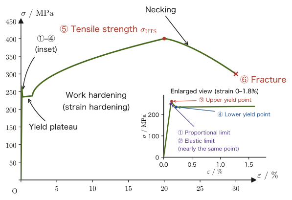
Example 19.6: Reading characteristic points from a stress–strain diagram
Looking at the stress–strain diagram in Figure 19.5, answer the following: (1) the name of the stress peak that appears first after the proportional limit is exceeded; (2) the type of deformation occurring in the material in the interval where the stress hardly changes and only the strain advances; (3) the name of the highest point of the curve.
Solution. (1) The small peak that appears immediately after the proportional limit is exceeded is the upper yield point. (2) In the subsequent interval in which the stress is almost constant while only the strain increases (the yield plateau), the material undergoes not elastic deformation but plastic deformation (permanent deformation that does not return to the original state even after unloading; the opposite of “elasticity” seen in Definition 18.4 in Section 18.1). (3) The highest point of the curve is the tensile strength (ultimate strength), which represents the maximum stress that the material can withstand in the sense of nominal stress (these definitions are treated in more detail in Section 19.5).
Application: Unit conversion — Pa, MPa, and GPa
In SI units the unit of stress is $\mathrm{Pa}=\mathrm{N/m^2}$, but the magnitudes of stress that actually occur in the mechanics of materials (the Young's modulus of steel is about $2\times10^{11}\ \mathrm{Pa}$, and its strength about $10^{8}\ \mathrm{Pa}$) are very large numbers, so in practice it is usual to use $\mathrm{MPa}=10^{6}\ \mathrm{Pa}=\mathrm{N/mm^2}$ (megapascal) and $\mathrm{GPa}=10^{9}\ \mathrm{Pa}$ (gigapascal). The relation $\mathrm{MPa}=\mathrm{N/mm^2}$ in particular is convenient: if the cross-sectional area of the specimen is measured in $\mathrm{mm^2}$ and the load is kept in $\mathrm N$, the stress is obtained directly in $\mathrm{MPa}$ ($\mathrm{N/mm^2}=\mathrm N/(10^{-3}\,\mathrm m)^2=10^{6}\,\mathrm{N/m^2}=\mathrm{MPa}$). From here on in this chapter as well, we often use $\mathrm{MPa}$ so that the numbers are easy to read.
19.5 Advanced Topic: Details of the Stress–Strain Diagram and True Stress and True Strain
Beyond the proportional limit lies important information that bears directly on the design of structures: yielding, tensile strength, and fracture. In this section we define in turn each point (①–⑥) of the stress–strain diagram of mild steel in Figure 19.5, and then go on to look at the difference between the two kinds of stress and strain, “nominal” and “true,” and at the contrast with brittle materials such as ceramics.
19.5.1 Definitions of the points on the stress–strain diagram
Definition 19.8: Elastic limit
The upper limit of stress (② in Figure 19.5) up to which the strain returns completely to 0 when the load is removed (no permanent deformation remains) is called the elastic limit $\sigma_{\mathrm e}\ [\mathrm{Pa}]$. In mild steel, the elastic limit is so close to the proportional limit $\sigma_{\mathrm p}$ that the two are almost indistinguishable (Figure 19.5 draws them as nearly the same point). The definitions themselves, however, differ—the proportional limit is a quantity determined by the shape of the graph, namely whether it is a straight line, whereas the elastic limit is a quantity determined by reversibility, namely whether the material returns to its original state after unloading—and in general $\sigma_{\mathrm e}\ge\sigma_{\mathrm p}$ (because even when the graph has just begun to deviate slightly from the straight line, the material may still recover completely elastically).
Definition 19.9: Upper and lower yield points
Beyond the elastic limit, the material begins to undergo plastic deformation (permanent deformation). In some metals such as mild steel, a characteristic behavior is observed: immediately after plastic deformation begins, the stress temporarily forms a sharp peak and then drops suddenly. This peak (③ in Figure 19.5) is called the upper yield point $\sigma_{\mathrm{yu}}$, and the point at which the stress then settles (④ in Figure 19.5) is called the lower yield point $\sigma_{\mathrm{yl}}$. After the lower yield point, there follows for a while a stretch in which the strain alone advances with the stress hardly changing (the yield plateau). During the yield plateau, plastic deformation does not occur uniformly throughout the specimen; instead, a deformed band called a Lüders band spreads over the specimen from one end to the other.
Intuition: Why a peak appears at the yield point
In crystalline metals such as mild steel, plastic deformation proceeds by the motion of “dislocations” (a dislocation is a line-shaped defect in a crystal where the arrangement of atoms is shifted by one row) through the crystal. Before yielding begins, the dislocations are slightly anchored (pinned) in their surroundings by impurities such as carbon atoms. To start moving a dislocation, an extra stress is needed that is large enough to break away from this pinning, and this is what the “peak” of the upper yield point really is. Once the dislocations start to move, they are released from the pinning and move more easily, so the stress falls to the lower yield point. During the yield plateau, the dislocations that are already moving propagate through the crystal, and the plastic deformation spreads. Not all metals show this phenomenon; in many metals (such as aluminum alloys) neither an upper nor a lower yield point appears, and the behavior passes smoothly from the elastic region to the plastic region.
For metals in which the upper and lower yield points do not appear clearly (many nonferrous metals and alloys), the proof stress, defined as follows, is used instead of the “yield point” as a guide to the onset of plastic deformation.
Definition 19.10: Proof stress (0.2% offset method)
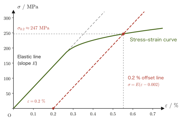
Draw the line obtained by shifting the elastic straight line through the origin of the stress–strain diagram parallel to itself by $0.2\%=0.002$ along the strain axis; the stress at the intersection of this line with the stress–strain curve is called the proof stress (often written $\sigma_{0.2}$). It means “the stress at which a permanent strain of 0.2% remains,” and is widely used in practice as a measure of yielding for materials that do not have a distinct yield point.
Definition 19.11: Tensile strength (ultimate strength)
After the yield plateau, the material becomes able to withstand more stress the more it deforms—this phenomenon is called work hardening (also called strain hardening). The nominal stress–nominal strain curve rises again, and after reaching a certain maximum value it begins to fall. The nominal stress at this maximum value (the top of the curve, ⑤ in Figure 19.5) is called the tensile strength or the ultimate strength $\sigma_{\mathrm{UTS}}$.
Definition 19.12: Fracture, elongation, and reduction of area
Beyond the tensile strength, part of the specimen becomes locally thinner (“necking,” treated in Section 19.5.3); the nominal stress decreases, and finally the specimen separates into two pieces (⑥ in Figure 19.5). This is called fracture. Letting $L_f$ be the gauge length at fracture, the quantities
$$ \text{elongation}=\frac{L_f-l_0}{l_0}\times100\ [\%],\qquad \text{reduction of area}=\frac{A_0-A_f}{A_0}\times100\ [\%] $$(where $A_f$ is the cross-sectional area at the fractured section) are, respectively, the representative quantities that express the ductility of a material (the property of deforming greatly before breaking). The larger the elongation and the reduction of area, the more ductile the material; the smaller they are (the material breaks with almost no deformation), the stronger its brittleness is said to be.
Example 19.7: Finding $E$, the proportional limit, the yield stress, the tensile strength, the elongation, and the reduction of area from tensile test data
A round steel bar of diameter $d=10.0\ \mathrm{mm}$ (cross-sectional area $A_0=\pi d^2/4=78.5\ \mathrm{mm^2}$) and gauge length $l_0=50.0\ \mathrm{mm}$ was subjected to a tensile test, and the following loads $P$ and elongations $\lambda$ between the gauge points were obtained. When the load reached $P=23\ \mathrm{kN}$, the elongation alone began to advance with almost no increase in load (the last entry of the table is a value partway through this stage); after that, the load reached the maximum load $P_{\max}=35\ \mathrm{kN}$, necking occurred, and the bar fractured. The gauge length after fracture was $L_f=65.0\ \mathrm{mm}$, and the diameter at the fractured section was $d_f=6.0\ \mathrm{mm}$.
| $P\ [\mathrm{kN}]$ | 0 | 5 | 10 | 15 | 20 | 22 | 23 |
|---|---|---|---|---|---|---|---|
| $\lambda\ [\mathrm{mm}]$ | 0 | 0.016 | 0.032 | 0.048 | 0.064 | 0.074 | 0.40 |
(1) Tabulate the nominal stress $\sigma=P/A_0\ [\mathrm{MPa}]$ and the nominal strain $\varepsilon=\lambda/l_0$ at each point. (2) Find Young's modulus $E$ from the slope of the straight portion. (3) Find the proportional limit $\sigma_{\mathrm p}$, the yield stress $\sigma_{\mathrm y}$, and the tensile strength $\sigma_{\mathrm{UTS}}$. (4) Find the elongation $[\%]$ and the reduction of area $[\%]$.
Solution. (1) $A_0=\pi\times10.0^2/4=78.54\ \mathrm{mm^2}$. If the load is used in $\mathrm N$ and the cross-sectional area in $\mathrm{mm^2}$, the stress comes out directly in $\mathrm{MPa}$ ($=\mathrm{N/mm^2}$) (see the Application in Section 19.4). For example, at the point $P=5\ \mathrm{kN}=5000\ \mathrm N$, $\sigma=5000/78.54=63.7\ \mathrm{MPa}$ and $\varepsilon=0.016/50.0=3.2\times10^{-4}$. Computing all the points gives the following table.
| $P\ [\mathrm{kN}]$ | $\sigma\ [\mathrm{MPa}]$ | $\varepsilon$ | $\sigma/\varepsilon\ [\mathrm{GPa}]$ |
|---|---|---|---|
| 0 | 0 | 0 | — |
| 5 | 63.7 | $3.2\times10^{-4}$ | 199 |
| 10 | 127.3 | $6.4\times10^{-4}$ | 199 |
| 15 | 191.0 | $9.6\times10^{-4}$ | 199 |
| 20 | 254.6 | $1.28\times10^{-3}$ | 199 |
| 22 | 280.1 | $1.48\times10^{-3}$ | 189 |
| 23 | 292.8 | $8.0\times10^{-3}$ | 36.6 |
(2) At the four points from $P=0$ to $20\ \mathrm{kN}$, $\sigma/\varepsilon$ is constant at $199\ \mathrm{GPa}$ in every case; that is, the points of $\sigma$–$\varepsilon$ lie on a straight line through the origin (Hooke's law). The slope of this line is $E$, and $E\approx199\ \mathrm{GPa}\approx2.0\times10^{2}\ \mathrm{GPa}$ (a representative value for steel, in agreement with Table 19.1).
(3) Proportional limit: up to the $20\ \mathrm{kN}$ point, the ratio is constant at $\sigma/\varepsilon=199\ \mathrm{GPa}$, but at the $22\ \mathrm{kN}$ point it is $189\ \mathrm{GPa}$, about $5\%$ smaller, so the data have begun to deviate from the straight line. Therefore the proportional limit that can be read from the data is $\sigma_{\mathrm p}\approx255\ \mathrm{MPa}$ (at least $255\ \mathrm{MPa}$ and less than $280\ \mathrm{MPa}$). Yield stress: at the point $P=23\ \mathrm{kN}$, where the elongation alone began to advance with almost no increase in load, $\sigma_{\mathrm y}=23000/78.54\approx293\ \mathrm{MPa}$. Tensile strength: dividing the maximum load $P_{\max}=35\ \mathrm{kN}$ by the cross-sectional area before deformation gives $\sigma_{\mathrm{UTS}}=35000/78.54\approx446\ \mathrm{MPa}$ (note that we divide by $A_0$, because this is the maximum value of the nominal stress).
(4) Elongation $=(L_f-l_0)/l_0\times100=(65.0-50.0)/50.0\times100=30\%$. The cross-sectional area at the fractured section is $A_f=\pi\times6.0^2/4=28.27\ \mathrm{mm^2}$, so the reduction of area $=(A_0-A_f)/A_0\times100=(78.54-28.27)/78.54\times100\approx64\%$. Since both the elongation and the reduction of area are large, we see that this steel is highly ductile.
Example 19.8: Finding the 0.2% proof stress
Suppose that the stress–strain curve of an aluminum alloy with Young's modulus $E=70\ \mathrm{GPa}$ is given as follows. In the elastic region ($\sigma\le\sigma_{\mathrm y}=180\ \mathrm{MPa}$), $\sigma=E\varepsilon$. Beyond it, in the plastic region, writing the total strain as $\varepsilon=\sigma/E+\varepsilon_{\mathrm{pl}}$ ($\sigma/E$ is the elastic strain and $\varepsilon_{\mathrm{pl}}$ is the plastic strain), $\sigma=\sigma_{\mathrm y}+H\varepsilon_{\mathrm{pl}}^{\,n}$ ($H=800\ \mathrm{MPa}$, $n=0.4$). Find the proof stress $\sigma_{0.2}$ by the 0.2% offset method.
Solution. In the 0.2% offset method, we draw the line $\sigma=E(\varepsilon-0.002)$ obtained by shifting the elastic straight line parallel to itself by $0.002$ along the strain axis (Figure 19.6), and find the stress at the intersection of this line with the stress–strain curve. Since the intersection $(\varepsilon^*,\sigma^*)$ lies on the curve, $\varepsilon^*=\sigma^*/E+\varepsilon_{\mathrm{pl}}$, and since it lies on the line, $\sigma^*=E(\varepsilon^*-0.002)$, that is, $\varepsilon^*-\sigma^*/E=0.002$. Comparing the two, we see that at the intersection the plastic strain is exactly $\varepsilon_{\mathrm{pl}}=0.002$ (0.2%)—this is the origin of the name “the stress at which a permanent strain of 0.2% remains.” Therefore, substituting $\varepsilon_{\mathrm{pl}}=0.002$ into the formula for the plastic region,
$$ \sigma_{0.2}=\sigma_{\mathrm y}+H\varepsilon_{\mathrm{pl}}^{\,n}=180+800\times0.002^{0.4}=180+800\times0.0833\approx247\ \mathrm{MPa} $$The strain at the intersection is $\varepsilon^*=\sigma_{0.2}/E+0.002=246.6/(70\times10^{3})+0.002\approx5.5\times10^{-3}$ ($0.55\%$). Note also that the offset line $\sigma=E(\varepsilon-0.002)$ gives $\sigma=0$ at $\varepsilon=0.002$, so it passes through the $0.2\%$ point of the strain axis.
19.5.2 Nominal stress and nominal strain, and true stress and true strain
The nominal stress $\sigma=P/A_0$ that we saw in Definition 19.6 is a quantity that keeps being divided by the cross-sectional area $A_0$ before deformation, even as the deformation proceeds. The stress actually felt at a point inside the specimen, however, should be $P/A$, obtained by dividing by the true cross-sectional area at each moment, $A$. In particular, in the latter half of the tensile test (after necking has progressed), the area $A$ of the narrowest cross section has become much smaller than $A_0$, so $P/A_0$ and $P/A$ take very different values.
Definition 19.13: True stress and true strain
The quantity defined, using the current cross-sectional area $A$ after the deformation has progressed (after necking has occurred, the area $A_{\min}$ of the narrowest cross section), by
\begin{equation} \sigma_{\mathrm t}=\frac{P}{A} \label{eq:19-true-stress} \end{equation}is called the true stress. As for strain, apart from the nominal strain obtained by dividing by the original length $l_0$, while the specimen is stretching uniformly, the quantity obtained by integrating, from the start of the deformation to the current length $L$, the infinitesimal rate of elongation $\dd L/L$ at each instant at which the length stretches from $L$ to $L+\dd L$,
\begin{equation} \varepsilon_{\mathrm t}=\int_{l_0}^{L}\frac{\dd L'}{L'}=\ln\frac{L}{l_0} \label{eq:19-true-strain} \end{equation}is called the true strain. After necking begins, the elongation between the gauge points cannot represent the behavior of the region where the deformation is concentrated. We therefore define $\varepsilon_{\mathrm t}=\ln(A_0/A_{\min})$ from the minimum cross-sectional area $A_{\min}$ at the neck (while the specimen is stretching uniformly, $A_0/A=L/l_0$ because the volume is constant, so this definition agrees with Eq. \eqref{eq:19-true-strain}).
Why?: The reason true strain is a logarithm
The nominal strain $\varepsilon=(L-l_0)/l_0$ is a quantity that measures “how much the specimen has stretched so far” all at once, with the length before deformation, $l_0$, as the reference. True strain, by contrast, is built on the following idea: “when the length is $L'$, if it stretches by a further $\dd L'$, the infinitesimal strain relative to the length $L'$ at that moment is $\dd L'/L'$”; these infinitesimal strains are summed (integrated) from the start of the deformation to the present. For a large deformation in which the length keeps changing, it is physically more natural to “always take the length at that moment as the reference,” and carrying out the integral $\int\dd L'/L'=\ln L+\text{constant}$ in Eq. \eqref{eq:19-true-strain} (the reverse of differentiating the logarithm, $\dd(\ln x)/\dd x=1/x$) naturally gives the logarithmic form. When the strain is small ($L\approx l_0$), the nominal strain and the true strain nearly coincide (we will confirm this in Example 19.9 below).
In the plastic deformation of metals, the atoms merely rearrange themselves and the volume hardly changes (the slight change in volume due to elastic deformation can be neglected). Therefore, while the specimen as a whole is stretching uniformly (until necking begins), we may set $AL=A_0l_0$ (constant volume), so that $A=A_0l_0/L=A_0/(1+\varepsilon)$, and the true stress and true strain can be rewritten in terms of the nominal stress and nominal strain.
Derivation: Relations between true stress and strain and nominal stress and strain
Note that the following relations hold only while the deformation is uniform between the gauge points (until necking begins, that is, up to the point of the tensile strength). From the constant volume $AL=A_0l_0$ we have $A_0/A=L/l_0=1+\varepsilon$. Using this in Eq. \eqref{eq:19-true-stress},
$$ \sigma_{\mathrm t}=\frac{P}{A}=\frac{P}{A_0}\cdot\frac{A_0}{A}=\sigma(1+\varepsilon) $$Also, substituting $L/l_0=1+\varepsilon$ into Eq. \eqref{eq:19-true-strain} gives
\begin{equation} \sigma_{\mathrm t}=\sigma(1+\varepsilon),\qquad \varepsilon_{\mathrm t}=\ln(1+\varepsilon) \label{eq:19-true-from-nominal} \end{equation}These are the same relations as those used in the simulator material “Fracture Mechanics” (fracture-derivation.html §1.1) (there the nominal strain is written $e$, but in this book we continue to use $\varepsilon$, which we have used consistently up to this point, for the nominal strain).
∎
Example 19.9: Calculating the true stress and true strain
In a certain tensile test, the nominal stress was $\sigma=350\ \mathrm{MPa}$ and the nominal strain was $\varepsilon=0.20$ ($20\%$). Find the true stress $\sigma_{\mathrm t}$ and the true strain $\varepsilon_{\mathrm t}$. Also, for comparison, find the true strain for a small nominal strain ($\varepsilon=0.001$), and compare how much it differs from the nominal strain.
Solution. From Eq. \eqref{eq:19-true-from-nominal},
$$ \sigma_{\mathrm t}=\sigma(1+\varepsilon)=350\times(1+0.20)=350\times1.20=420\ \mathrm{MPa} $$ $$ \varepsilon_{\mathrm t}=\ln(1+\varepsilon)=\ln(1.20)\approx0.1823 $$The true stress ($420\ \mathrm{MPa}$) is considerably larger than the nominal stress ($350\ \mathrm{MPa}$), and the true strain ($0.1823$) is slightly smaller than the nominal strain ($0.20$). On the other hand, for $\varepsilon=0.001$, $\varepsilon_{\mathrm t}=\ln(1.001)\approx0.0009995$, which nearly coincides with the nominal strain $0.001$ (this is why, in the range of small strain such as elastic deformation, we need not worry about the difference between nominal and true).
19.5.3 Work hardening, Hollomon's equation, and necking
An empirical formula is known that expresses quantitatively, in terms of the true stress and true strain, the work hardening described in Section 19.5.1—the phenomenon in which the further plastic deformation proceeds, the harder it becomes for the material to deform.
Law 19.2: Hollomon's equation
For many metals, the relation between the true stress and the true strain in the plastic deformation region is well approximated by the power function
\begin{equation} \sigma_{\mathrm t}=K_{\mathrm H}\varepsilon_{\mathrm t}^{\,n} \label{eq:19-hollomon} \end{equation}(Hollomon, 1945). $K_{\mathrm H}$ is called the strength coefficient and $n$ ($0\lt n\lt1$) the work-hardening exponent. A larger $n$ means a greater work-hardening effect (the material becomes harder more readily as the deformation proceeds). In the simulator material “Fracture Mechanics” (fracture-derivation.html §1.2) the strength coefficient is written $K$, but in this book it is written $K_{\mathrm H}$ to distinguish it from the bulk modulus $K$.
Even though work hardening is present, why does the nominal stress decrease once the tensile strength is exceeded? The answer is “necking.” Once the tensile strength is exceeded, an extremely slight variation in the cross-sectional area of the specimen (a perfectly uniform bar cannot be made in reality) triggers the deformation to begin concentrating at the location with the smallest cross-sectional area. This is necking.
Discussion: Why does necking begin at the point of tensile strength? — Considère's condition
Differentiating the load $P=\sigma_{\mathrm t}A$ with respect to the true strain $\varepsilon_{\mathrm t}$, and using the product rule (University Mathematics, Section 1.4) together with $\dd A/A=-\dd\varepsilon_{\mathrm t}$, which follows from the constant-volume condition (just differentiate $A=A_0e^{-\varepsilon_{\mathrm t}}$), we obtain
$$ \frac{\dd P}{\dd\varepsilon_{\mathrm t}}=A\frac{\dd\sigma_{\mathrm t}}{\dd\varepsilon_{\mathrm t}}+\sigma_{\mathrm t}\frac{\dd A}{\dd\varepsilon_{\mathrm t}}=A\left(\frac{\dd\sigma_{\mathrm t}}{\dd\varepsilon_{\mathrm t}}-\sigma_{\mathrm t}\right) $$At the maximum of the load (the point corresponding to the tensile strength), $\dd P/\dd\varepsilon_{\mathrm t}=0$; since $A\neq0$, the condition for necking to begin is therefore
\begin{equation} \frac{\dd\sigma_{\mathrm t}}{\dd\varepsilon_{\mathrm t}}=\sigma_{\mathrm t} \label{eq:19-considere} \end{equation}This is Considère's condition. That is, at the instant when “the slope of the tangent to the true stress–true strain curve (the work-hardening rate) becomes equal to the value of the true stress itself,” the load turns from increasing to decreasing, and beyond that point the deformation concentrates at a single location—this is the physical meaning of necking. In terms of the nominal stress $P/A_0=\sigma_{\mathrm t}A/A_0=\sigma_{\mathrm t}e^{-\varepsilon_{\mathrm t}}$, obtained by dividing the load by the initial cross-sectional area, we have
$$ \frac{\dd(P/A_0)}{\dd\varepsilon_{\mathrm t}}=e^{-\varepsilon_{\mathrm t}}\left(\frac{\dd\sigma_{\mathrm t}}{\dd\varepsilon_{\mathrm t}}-\sigma_{\mathrm t}\right) $$The fact that this derivative becomes negative ($\dd\sigma_{\mathrm t}/\dd\varepsilon_{\mathrm t}\lt\sigma_{\mathrm t}$) is the mathematical expression of the statement “the load decreases because the cross-sectional area shrinks faster than the strength grows through work hardening.” Substituting Hollomon's equation \eqref{eq:19-hollomon} gives $\dd\sigma_{\mathrm t}/\dd\varepsilon_{\mathrm t}=nK_{\mathrm H}\varepsilon_{\mathrm t}^{n-1}=(n/\varepsilon_{\mathrm t})\sigma_{\mathrm t}$, so Eq. \eqref{eq:19-considere} reduces to $n/\varepsilon_{\mathrm t}=1$; that is, the true strain at which necking begins is equal to the work-hardening exponent $n$ ($\varepsilon_{\mathrm t}=n$)—a simple result. For $\varepsilon_{\mathrm t}\gt n$ we have $\dd\sigma_{\mathrm t}/\dd\varepsilon_{\mathrm t}\lt\sigma_{\mathrm t}$, and the load decreases. The details of this derivation are given in the simulator material “Fracture Mechanics” (fracture-derivation.html §1.3), where the same result is obtained.
After necking begins, the stress distribution within the specimen is no longer uniform—the central region of the narrowest cross section of the neck receives tensile stress not only in the tensile direction but also in the transverse directions, because the thicker surrounding portions prevent lateral contraction. Such a state in which stress acts in all three directions is called a triaxial stress state. As a result, the mean stress at the minimum cross section,$\bar\sigma=P/A_{\min}$, is estimated to be higher than the true flow stress $\sigma_{\mathrm{eq}}$ (the value under the assumption of uniform tension). The correction that compensates for this effect is the Bridgman correction. Let $a$ be the radius of the minimum cross section of the neck and $R$ the radius of curvature of the neck profile; then the correction factor is given by $B=(1+2R/a)\ln(1+a/2R)\ (\ge1)$ and $\sigma_{\mathrm{eq}}=\bar\sigma/B$. As $R/a$ becomes larger (the gentler the neck), $B\to1$ and the correction becomes unnecessary; the sharper the neck (the smaller $R/a$), the larger the correction becomes. We do not go into the derivation of this correction in this book. An outline of what happens after necking that leads to fracture (the formation, growth, and coalescence of voids—tiny cavities that form inside the material) is given in Section 21.7.
19.5.4 Ductile fracture and brittle fracture, and the contrast with ceramics
The sequence “elastic deformation → yielding → work hardening → necking → fracture” seen so far is behavior characteristic of ductile materials such as steel and aluminum. They do not break immediately even when the tensile strength is exceeded, but fracture only after large plastic deformation (elongation and reduction of area); a visible warning in the form of “large deformation” therefore appears before a structure fails.
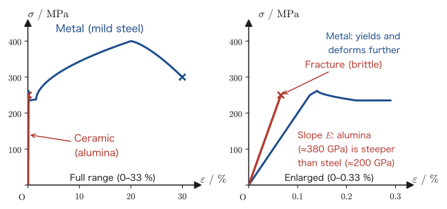
In contrast, brittle materials such as glass and alumina (aluminum oxide, a representative ceramic) show no yielding, and the straight line of elastic deformation continues unchanged until fracture. In this case the tensile strength is the fracture stress itself, and fracture occurs suddenly without warning. Note that ceramics are weak in tension but strong in compression (in compression, the force acts in the direction that closes cracks, so cracks have difficulty spreading). The reason metals and ceramics behave so differently lies in the difference in bonding at the atomic and molecular level. Metallic bonding is like metal ions immersed in a “sea of electrons” that is not strongly tied to any particular pair of atoms, so dislocations move relatively easily and plastic deformation (deformation in which atomic planes slip while the crystal structure is preserved) occurs readily. On the other hand, the situation is different for covalent bonds and ionic bonds, which account for most ceramics. A covalent bond is strongly directional along particular directions, so to move a dislocation, bonds must be broken and rearranged. An ionic bond has no directionality, but when atomic planes slip, ions of the same sign come to be adjacent and Coulomb repulsion arises, so slip is difficult. Consequently, in both cases dislocations hardly move at room temperature, and with almost no plastic deformation the interatomic bonds break immediately after elastic deformation (the mechanism by which bonds break is studied in detail in Chapter 21).
Application: Young's modulus and Poisson's ratio of representative materials
Young's modulus $E$ and Poisson's ratio $\nu$ are basic material properties that are the first to be consulted when selecting a material. Approximate values for representative materials are given in Table 19.1.
| Material | $E\ [\mathrm{GPa}]$ | $\nu$ | $G\ [\mathrm{GPa}]$ | $K\ [\mathrm{GPa}]$ | Tensile strength $[\mathrm{MPa}]$ |
|---|---|---|---|---|---|
| Steel (mild steel, structural steel) | 200–210 | 0.28–0.30 | about 80 | about 160 | 400–550 |
| Aluminum alloy | 69–73 | 0.33 | about 27 | about 70 | about 310 (6061-T6) |
| Copper | 110–128 | 0.33–0.36 | about 44 | about 120 | about 220 (annealed) |
| Soda-lime glass | 65–72 | 0.20–0.23 | about 29 | about 42 | several tens (strongly dependent on surface flaws) |
| Alumina (polycrystalline $\mathrm{Al_2O_3}$) | 350–400 | 0.21–0.27 | about 156 | about 230 | about 200–300 |
| Diamond | about 1000 | — | — | — | — |
| Rubber | 0.001–0.1 | about 0.5 | — | — | — |
| Wood (along the grain) | 10–16 | — | — | — | — |
| Polyethylene | about 1 (depends on the type) | — | — | — | — |
The values in the table are representative values found in the textbook by Callister et al. (Reference 4) and other sources, and they can scatter by several tens of percent from the tabulated values depending on the composition of the alloy, the heat treatment, the porosity (in the case of ceramics), and so on. The tensile strength in particular covers a wide range and is only a guide to the order of magnitude. When using these values in design, one must always check the data sheet of the material itself. $G,K$ were obtained by substituting representative values of $E$ and $\nu$ (steel $205\ \mathrm{GPa}$ and $0.29$, aluminum alloy $71\ \mathrm{GPa}$ and $0.33$, copper $119\ \mathrm{GPa}$ and $0.34$, glass $70\ \mathrm{GPa}$ and $0.22$, alumina $380\ \mathrm{GPa}$ and $0.22$) into Formula 19.1 and Formula 19.2. For diamond, rubber, wood, and polyethylene, only the approximate value of $E$, which is used in Exercise 19.6, is given (entries for materials that are not isotropic, or for which $\nu$ is hard to determine, are left blank).
When we compare the metals (steel, aluminum, copper), Young's modulus reflects the strength of the interatomic bonds, and in general the higher the melting point of a metal, the higher its Young's modulus tends to be. Ceramics (alumina), reflecting the strength of covalent and ionic bonds, often have a larger Young's modulus than metals (Figure 19.7). However, their tensile strength is smaller than that of metals—being “hard” and being “brittle” at the same time are two sides of the same coin, as we saw in Section 19.5.4.
Application: The atomistic origin of the elastic modulus
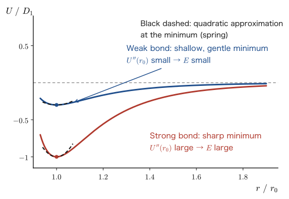
Recall the potential energy curve $U(r)$ as a function of the interatomic distance $r$ (a Lennard-Jones-type potential, etc.), which we saw in Section 4.6, “Application: Interatomic potential and bond length.” The atoms stay near the equilibrium distance $r_0$ at which $U(r)$ takes its minimum value (a stable equilibrium point in the sense of Theorem 4.4 of Chapter 4). If an external force changes the interatomic distance slightly from $r_0$ by $x=r-r_0$, the interatomic force can be approximated as
$$ f(r)=-\frac{\dd U}{\dd r}\approx-\frac{\dd U}{\dd r}\bigg|_{r_0}-\left.\frac{\dd^2U}{\dd r^2}\right|_{r_0}x=-\left.\frac{\dd^2U}{\dd r^2}\right|_{r_0}x $$where we used the Taylor expansion (University Mathematics, Section 4.2) and the fact that $r_0$ is a minimum point, so that $\dd U/\dd r|_{r_0}=0$. This is precisely the form of Hooke's law $f=-kx$, and the quantity corresponding to the spring constant is the curvature (second derivative) of the potential curve at its bottom, $k=\dd^2U/\dd r^2|_{r_0}$.
How, then, is the macroscopic Young's modulus $E$ determined from this microscopic spring constant $k$? Let us estimate it with a simple model in which the atoms are arranged in a cubic lattice with edge length $r_0$. The cross-sectional area carried by a single row of atoms (a chain of bonds) is $r_0^2$. When the interatomic distance is stretched by $x$, the force in one bond is $kx$, the strain is $\varepsilon=x/r_0$, and the stress is the force per bond divided by the area it carries, $\sigma=kx/r_0^2$. Therefore we obtain
\begin{equation} E=\frac{\sigma}{\varepsilon}=\frac{kx/r_0^{2}}{x/r_0}=\frac{k}{r_0}=\frac{1}{r_0}\left.\frac{\dd^2U}{\dd r^2}\right|_{r_0} \label{eq:19-E-atomic} \end{equation}(Allowing for the crystal structure and the directions of the bonds produces deviations of a factor of several, but the order of magnitude is correct.) For example, for iron ($E=2\times10^{11}\ \mathrm{Pa}$, nearest-neighbor interatomic distance $r_0\approx2.5\times10^{-10}\ \mathrm{m}$), $k=Er_0\approx50\ \mathrm{N/m}$, which is much stiffer than a coil spring on a desk (a few $\mathrm{N/m}$). Eq. \eqref{eq:19-E-atomic} shows that the elastic modulus is nothing other than how sharply the bottom of the interatomic potential curves, measured on a macroscopic scale (Figure 19.8). The Young's modulus of a material is larger the stronger its bonds are and the more sharply and steeply the bottom of its potential rises (the larger its curvature). That the Young's modulus of diamond (whose covalent bonds are extremely strong and directional) exceeds $E\approx1000\ \mathrm{GPa}$, while that of polymer materials such as polyethylene, whose molecules are held together only by weak van der Waals forces, remains at about $E\sim1\ \mathrm{GPa}$, is due precisely to this difference in bond strength (the curvature of the potential).
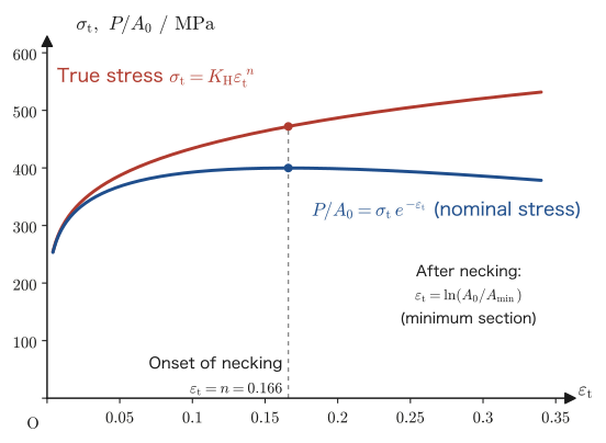
Example 19.10: Discrepancy between nominal stress and true stress (necking region)
Suppose that a mild steel can be approximated by Hollomon's equation \eqref{eq:19-hollomon} with $K_{\mathrm H}=636\ \mathrm{MPa}$ and $n=0.166$. (1) Find the true strain $\varepsilon_{\mathrm t}$ at which necking begins and the nominal strain $\varepsilon$ at that moment. (2) Find the true stress $\sigma_{\mathrm t}$ and the nominal stress $\sigma$ at the point where necking begins, and compare them. (3) When necking has progressed and the true strain at the minimum cross section has become $\varepsilon_{\mathrm t}=0.30$, find the true stress $\sigma_{\mathrm t}$ and the quantity $P/A_0$, the load divided by the initial cross-sectional area.
Solution. (1) By Considère's condition (a consequence of Eq. \eqref{eq:19-considere}), the true strain at which necking begins is $\varepsilon_{\mathrm t}=n=0.166$. From the inverse of the relation \eqref{eq:19-true-from-nominal}, which holds while the specimen elongates uniformly, we have $1+\varepsilon=e^{\varepsilon_{\mathrm t}}$, so the nominal strain is
$$ \varepsilon=e^{0.166}-1\approx1.1806-1=0.1806\approx18.1\% $$(2) From Hollomon's equation \eqref{eq:19-hollomon}, the true stress is
$$ \sigma_{\mathrm t}=K_{\mathrm H}\varepsilon_{\mathrm t}^{\,n}=636\times0.166^{0.166}\approx636\times0.7422\approx472\ \mathrm{MPa} $$Solving Eq. \eqref{eq:19-true-from-nominal}, $\sigma_{\mathrm t}=\sigma(1+\varepsilon)$, for $\sigma$ gives
$$ \sigma=\frac{\sigma_{\mathrm t}}{1+\varepsilon}=\frac{472}{1.1806}\approx400\ \mathrm{MPa} $$At the point where necking begins (the highest point of the nominal stress–nominal strain curve, that is, the tensile strength), the true stress ($\approx472\ \mathrm{MPa}$) is already about $18\%$ higher than the nominal stress ($\approx400\ \mathrm{MPa}$, which corresponds to the tensile strength $\sigma_{\mathrm{UTS}}$).
(3) At the minimum cross section of the neck, $A=A_0e^{-\varepsilon_{\mathrm t}}$ (Definition 19.13) and $P=\sigma_{\mathrm t}A$, so $P/A_0=\sigma_{\mathrm t}e^{-\varepsilon_{\mathrm t}}$. For $\varepsilon_{\mathrm t}=0.30$ (assuming that Hollomon's equation also holds in the neck),
$$ \sigma_{\mathrm t}=636\times0.30^{0.166}\approx521\ \mathrm{MPa},\qquad \frac{P}{A_0}=521\times e^{-0.30}\approx386\ \mathrm{MPa} $$Although the true stress is still increasing, $472\to521\ \mathrm{MPa}$, the load divided by $A_0$ is decreasing, $400\to386\ \mathrm{MPa}$. This is because the cross-sectional area $A$ decreases faster than the true stress grows through work hardening (see Figure 19.9).
19.6 Summary and Exercises
19.6.1 Summary
- Hooke's law (Law 19.1): Within the elastic range, stress and strain are directly proportional, and the constant of proportionality is called an elastic modulus. The ratio of normal stress to longitudinal strain is Young's modulus (modulus of longitudinal elasticity) $E$ (Definition 19.1), the ratio of shear stress to shear strain is the shear modulus (modulus of transverse elasticity) $G$ (Definition 19.2), and the ratio of hydrostatic normal stress to volumetric strain is the bulk modulus $K$ (Definition 19.3). For tension of a round bar, $E=l_0P/(\lambda A_0)$ (Eq. \eqref{eq:19-E-def}), and the bar can be regarded as a spring with spring constant $k=EA_0/l_0$ (Eq. \eqref{eq:19-bar-spring}).
- From the generalized Hooke's law (Eq. \eqref{eq:19-generalized-hooke}) we obtain $G=E/\{2(1+\nu)\}$ (Formula 19.1) and $K=E/\{3(1-2\nu)\}$ (Formula 19.2). For an isotropic elastic body only two elastic constants are independent ($E,\nu$ are also determined from $G,K$), and the range of possible values of $\nu$ is $-1\lt\nu\lt1/2$.
- Material testing is classified into static-load tests (tension, compression, torsion, flexure, hardness, creep) and dynamic-load tests (fatigue, impact), and is specified in detail by the Japanese Industrial Standards (JIS). The nominal stress is $\sigma=P/A_0$ (Definition 19.6), and the proportional limit is $\sigma_{\mathrm p}$ (Definition 19.7). The stress–strain diagram of mild steel follows a characteristic shape consisting of the proportional limit, elastic limit, upper and lower yield points, yield plateau, work hardening, tensile strength, necking, and fracture (Figure 19.5).
- For materials without a distinct yield point, the 0.2% proof stress (Definition 19.10) is used. In contrast to the nominal stress and nominal strain, which are obtained by dividing by the cross-sectional area before deformation, the true stress and true strain (Definition 19.13), which are obtained by dividing by the cross-sectional area at each instant, are related by $\sigma_{\mathrm t}=\sigma(1+\varepsilon)$ and $\varepsilon_{\mathrm t}=\ln(1+\varepsilon)$ (Eq. \eqref{eq:19-true-from-nominal}) as long as the specimen stretches uniformly (until necking begins). Work hardening is well approximated by Hollomon's equation $\sigma_{\mathrm t}=K_{\mathrm H}\varepsilon_{\mathrm t}^{\,n}$ (Law 19.2; the strength coefficient is written $K_{\mathrm H}$ to distinguish it from the bulk modulus $K$), and from Considère's condition $\dd\sigma_{\mathrm t}/\dd\varepsilon_{\mathrm t}=\sigma_{\mathrm t}$ (Eq. \eqref{eq:19-considere}) it follows that necking begins at the true strain $\varepsilon_{\mathrm t}=n$.
- Metals (ductile materials) fracture after large plastic deformation, whereas ceramics (brittle materials) remain in elastic deformation and fracture almost linearly (Figure 19.7)—this reflects the difference between metallic bonding on the one hand and, on the other, strongly directional covalent bonding or ionic bonding, in which slip brings ions of the same sign next to each other. Microscopically, Young's modulus corresponds to the curvature at the bottom of the interatomic potential curve (Chapter 4, Eq. \eqref{eq:19-E-atomic}).
Related simulator: Fracture Mechanics (Griffith and Weibull) and the corresponding derivation page (you can check the continuation of the nominal stress, true stress, Hollomon's equation, Considère's condition, and the stress inside the neck treated in this chapter by simulating an actual tensile test; the simulator writes the strength coefficient as $K$; it is used in earnest in Chapters 21 and 22).
19.6.2 Exercises
Exercise 19.1: Calculating Young's modulus
A load $P=1.0\times10^{4}\ \mathrm N$ is applied to a bar of cross-sectional area $A_0=5.0\times10^{-5}\ \mathrm{m^2}$ and length $l_0=2.0\ \mathrm{m}$, and the bar stretches by $\lambda=2.0\ \mathrm{mm}$. Find Young's modulus $E$ of this bar. Also, by comparing with the values in Table 19.1, answer what material the bar is likely to be made of.
Hint: Substitute the numbers directly into Eq. \eqref{eq:19-E-def} ($E=l_0P/(\lambda A_0)$). It is best to convert all quantities to SI units (m, N, Pa) before calculating.
Exercise 19.2: Finding $G,K$ from $E,\nu$
The Young's modulus of a certain copper alloy is $E=120\ \mathrm{GPa}$ and its Poisson's ratio is $\nu=0.35$. Find the shear modulus $G$ and the bulk modulus $K$.
Hint: Substitute the numbers directly into Formulas 19.1 and 19.2. Also check whether $\nu=0.35$ lies within the range $-1\lt\nu\lt0.5$ stated in Section 19.3.4.
Exercise 19.3: Equivalent modulus of bars connected in series
Two kinds of bars with equal cross-sectional area and equal length (Young's moduli $E_1,E_2$) are joined end to end, with the cross-sectional area unchanged, into a single bar, and a load $P$ is applied to the whole. Express the (apparent) Young's modulus $E_{\mathrm{eq}}$ of the combined bar as a whole in terms of $E_1,E_2$.
Hint: Use the analogy between “a bar stretches” and “a spring stretches.” Recall that when springs with spring constants $k_1,k_2$ are connected in series, the equivalent spring constant satisfies $1/k_{\mathrm{eq}}=1/k_1+1/k_2$ (a formula from high school physics), and focus on the spring constant of a bar, $k=P/\lambda=EA_0/l_0$ (Eq. \eqref{eq:19-bar-spring}). Use the fact that the sum of the elongations $\lambda_1,\lambda_2$ of the two bars is the elongation of the whole.
Exercise 19.4: Why the true stress keeps increasing even after necking
Even after the tensile strength (the highest point of the nominal stress–nominal strain curve) is passed, the true stress–true strain curve (Hollomon's equation) continues to increase monotonically, yet the quantity $P/A_0$ obtained by dividing the load by the initial cross-sectional area (the nominal stress) decreases. Using the load $P=\sigma_{\mathrm t}A$ and the change of the cross-sectional area at constant volume, $A=A_0e^{-\varepsilon_{\mathrm t}}$, explain this seemingly contradictory fact qualitatively.
Hint: Differentiate $P/A_0=\sigma_{\mathrm t}e^{-\varepsilon_{\mathrm t}}$ with respect to $\varepsilon_{\mathrm t}$, use Hollomon's equation $\sigma_{\mathrm t}=K_{\mathrm H}\varepsilon_{\mathrm t}^{\,n}$, and find where the sign changes. Consider which one “wins”: the decrease of the cross-sectional area or the increase of strength due to work hardening. The numbers in Example 19.10 may also be helpful.
Exercise 19.5: Classification of material tests
Classify the following eight material tests—the tensile test, compression test, torsion test, flexural test, hardness test, creep test, fatigue test, and impact test—into static-load tests and dynamic-load tests, and explain in a phrase what each test is intended to measure (its purpose).
Hint: Review the classification in Definition 19.5. Note that the “creep test” examines the slowly progressing deformation when a constant load is applied for a long time (even though the load itself is constant, it differs somewhat in character from the other static-load tests in that it involves a time element, namely long duration).
Exercise 19.6: Relative magnitudes of the Young's moduli of familiar materials (advanced problem)
Arrange the four materials rubber, steel, glass, and wood (along the grain) in order of increasing Young's modulus, and explain the reason for this order in terms of the type of bonding and the structure at the atomic and molecular level (see Section 19.5.4 and the “Application” at the end of Section 19.5). Then compare with Table 19.1 and values in the literature, and check to what extent your prediction was correct.
Hint: Rubber has a structure in which long hydrocarbon chains (polymers) are loosely entangled, and most of its deformation comes from the untangling of the chains (not from stretching the bonds themselves). Steel has metallic bonding, glass is a network structure based mainly on covalent bonds, and in wood (along the grain) the covalent bonds along the fibers, in which cellulose molecules are aligned, are what matter. Think of it this way: the more a deformation directly stretches bonds, the larger the Young's modulus tends to be.
19.6.3 References
- Yasuhide Mochizuki, Physics Notes: Mechanics of Materials (handwritten lecture notes, in Japanese). The source of this chapter (pp. 5–6).
- S. P. Timoshenko, D. H. Young, Elements of Strength of Materials, 5th ed., Van Nostrand, 1968.
- R. C. Hibbeler, Mechanics of Materials, 10th ed., Pearson, 2017.
- W. D. Callister, D. G. Rethwisch, Materials Science and Engineering: An Introduction, 10th ed., Wiley, 2018.
- Japanese Industrial Standards (JIS) Z 2241:2022, “Method of Tensile Test for Metallic Materials” (formerly Japanese Industrial Standard; in Japanese).