Chapter 18Fundamentals of Mechanics of Materials — Loads, Stress, and Strain
What you will be able to do after this chapter. You will be able to estimate numerically, units included, how much “force density” (stress) arises inside a material when a force is applied to a rod or a bolt, and how much the material changes shape (strain). In worked examples such as steel rods, concrete columns, and ceramic parts, you will actually compute values in the unit $\mathrm{MPa}$.
Why it is needed. Up to this point, in Parts I and II, we have treated a body either as a “point whose size can be neglected” (a particle, or point mass) or as a “hard lump whose shape does not change” (a rigid body). In reality, however, the steel frame of a bridge, the pillars of a building, and the ceramic parts inside a smartphone all deform slightly when a force acts on them. The discipline that does not ignore this “slight deformation” and asks up to what force a material can safely be used, and how far it can deform before it breaks, is mechanics of materials. Even if we create a new material, unless we can evaluate quantitatively how much force it can withstand, it cannot be used in actual parts or structures.
Connection to high school physics. In high school physics you should also have learned pressure $p=F/A$ (the force divided by the area) and Hooke's law $F=-kx$ (the restoring force of a spring is proportional to its extension). It is helpful to think of mechanics of materials as extending these two ideas—“divide the force by the area” and “deformation is proportional to force”—from the special component called a spring to the deformation of all solids in general, including metals, ceramics, and concrete. In this chapter we define “dividing the force by the area” (stress) and “dividing the deformation by the original length” (strain); the fact that the two are “proportional” is treated in the next chapter.
- Chapter 18 (this chapter) Fundamentals of mechanics of materials—the basic assumptions for thinking about mechanics of materials, the classification of loads, the definitions of stress (normal stress and shear stress) and strain, and Poisson's ratio.
- Chapter 19 Hooke's law, elastic moduli, and material testing—Young's modulus (modulus of longitudinal elasticity) $E$, shear modulus (modulus of transverse elasticity) $G$, and bulk modulus $K$, all of which link stress and strain, and the stress–strain diagram.
- Chapter 20 Multiaxial stress, bending of beams, and torsion—the case where forces act from several directions rather than just one, the bending stress of a beam, and the torsional stress of a shaft.
- Chapter 21 Fundamentals of fracture mechanics—why a material with a crack becomes weaker, the Griffith theory, and fracture toughness.
- Chapter 22 Fatigue, scatter in strength, and environment-assisted fracture—fatigue fracture due to repeated loads, the scatter in the strength of ceramics (Weibull statistics), and fracture in which the environment plays a part.
- How mechanics of materials models a solid—the seven basic assumptions (homogeneous body, isotropic body, internal forces, elasticity and plasticity, small deformation, the principle of superposition, and Saint-Venant's principle)
- The three ways of classifying loads (external forces)—by how they act (tension, compression, shear, torsion, bending), by how they are distributed (concentrated, distributed), and by how they vary in time (static, dynamic)
- The definitions of normal stress $\sigma=P/A$ and shear stress $\tau=Q/A$, the method of sections for finding the internal force, the sign convention (tension positive, compression negative), and the relations among the unit $\mathrm{Pa}=\mathrm{N/m^2}$, the $\mathrm{MPa}=\mathrm{N/mm^2}$ commonly used in engineering practice, and $\mathrm{GPa}$
- The definitions of longitudinal strain $\varepsilon=\Delta l/l_0$ and transverse strain $\varepsilon'$, and Poisson's ratio $\nu=\abs{\varepsilon'/\varepsilon}$ and Poisson's number $m=1/\nu$
- The definitions of shear strain $\gamma=\tan\alpha$ and volumetric strain $\varepsilon_V=\Delta V/V$, the idea of the first-order approximation for small deformations, and $\varepsilon_V\approx\varepsilon(1-2\nu)$ for uniaxial tension
Source notes: Yasuhide Mochizuki, Physics Notes: Mechanics of Materials, pp. 1–4.
18.1 Basic Assumptions of Mechanics of Materials and Internal Forces
Real metals and ceramics have an extremely complicated internal structure made up of atoms and crystal grains. Under magnification, grain boundaries (the interfaces between crystal grains) and tiny voids and impurities are found everywhere, and it is not unusual for hardness and the ease with which the material stretches to vary with the orientation of the crystal. However, if we tried to incorporate all of this complexity into equations, practical calculation would become almost impossible. Therefore, in mechanics of materials we simplify real materials into models that are easy to handle, in the same spirit in which we introduced the model of the “particle (point mass)” in Chapter 1 and that of the “rigid body” in Chapter 10. The following (i)–(vii) are the basic assumptions that underlie the whole discussion of mechanics of materials. We number the box titles with (i)–(vii) and summarize them at the end in Table 18.1.
Definition 18.1: Homogeneous body — Basic assumption (i)
We assume that the material is a continuous solid with no defects or cavities inside and that every part has the same properties. Such a material is called a homogeneous body. Real materials have a fine microstructure such as crystal grains, but when the dimensions of a member are sufficiently larger than the size of that microstructure, we may regard the material as a continuum packed without any gaps and approximate it as having the same properties in every part.
Definition 18.2: Isotropic body — Basic assumption (ii)
We assume that the mechanical properties of the material (such as how easily it stretches and how strong it is) do not change with the direction in which we look. Such a material is called an isotropic body. It is the property of being uniform, with mechanical properties such as strain independent of direction.
Caution: Anisotropic materials also exist (proviso to basic assumption (ii))
In some cases we also deal with anisotropic materials, whose mechanical properties differ with direction. For example, wood differs greatly in strength between the direction along the fibers and the direction perpendicular to them, and fiber-reinforced composite materials such as carbon-fiber-reinforced plastic (CFRP) are designed so that their properties vary with the orientation of the fibers. A metal, too, shows direction-dependent properties (anisotropy) if we take out just a single crystal grain (a single crystal), but when averaged over a polycrystal, in which many crystal grains with random orientations are gathered together, it behaves, on average, almost isotropically. In this book, unless otherwise stated, we proceed on the assumption that the material is the homogeneous, isotropic elastic body of Definition 18.1 and Definition 18.2.
Definition 18.3: Internal force — Basic assumption (iii)
When an external force acts on a material, a force that tries to resist that external force arises inside the material. This is called an internal force. The method of actually finding the magnitude of the internal force (the method of sections) is described in Section 18.3.
Intuition: Internal forces and Newton's third law
An internal force is not a special force that suddenly springs up from nowhere. If we imagine dividing the material into many tiny parts (clusters of atoms and molecules), neighboring parts exert pulling and pushing forces on one another. When no external force is applied, these forces are exactly balanced and the material does not deform. When an external force is applied, the balance of the forces between neighboring parts is upset, and the material deforms until it settles into a new equilibrium while the parts exert forces on their neighbors—this is the true nature of an internal force. Consider a cross section: the force that one side of the material exerts on the other side across that section and the force that the other side exerts on the first side have, by the law of action and reaction (Section 2.3), equal magnitudes and opposite directions. The “stress” defined in the next Section 18.3 is this internal force divided by the area of the cross section and expressed as a “density” of force.
Paired with the property that an internal force arises when an external force acts on a material is the nature of the deformation itself. We classify materials as follows, according to how they recover (or fail to recover) from the deformation after being subjected to an external force.
Definition 18.4: Elasticity and plasticity — Basic assumption (iv)
The property of returning to the original shape, with the deformation disappearing, when the external force is removed is called elasticity. In this book we deal in particular with elasticity in which the deformation caused by the external force is proportional to the magnitude of the force (linear elasticity). Conversely, the property that deformation remains even after the external force is removed is called plasticity.
Intuition: Examples of elasticity and plasticity from high school physics
A familiar example of elasticity is the coil spring you studied in high school physics. If you pull a spring a little and let go, it returns to its original length—this is elasticity. On the other hand, if you bend a wire a great deal, it stays bent when you let go and does not return to its original shape. This is plastic deformation. In general, any material behaves elastically while the external force (and hence the deformation) is small, and once the external force exceeds a certain limit (the elastic limit), plastic deformation remains. In this chapter and the next (Chapter 19) we deal mainly with the elastic range only. The details of plastic deformation and of the transition from elastic to plastic behavior are treated in Chapter 19, in connection with the stress–strain diagram. Note that “returning to the original state” and “the deformation being proportional to the force” are separate properties. Rubber returns to its original state when released even after being stretched a lot (elasticity), but its elongation is not proportional to the force (nonlinear elasticity). What basic assumption (iv) requires is linear elasticity, in which the material both returns to its original state and deforms in proportion to the force; this holds for many materials when the deformation is small.
Caution: The small-deformation assumption — Basic assumption (v)
In mechanics of materials we assume that the deformation of a material due to external forces is extremely small, and that the deformation does not change the way the external forces act (the positions and directions at which the forces are applied). For example, this means that even if we pull a bar and it stretches slightly, the direction in which the force is applied and the cross-sectional area that bears the force change only by amounts negligible in the calculation. Thanks to this assumption, we can treat the relation between force and deformation as linear (a proportional relation), and the principle of superposition described next also holds. When the deformation actually becomes large (for example, when rubber is stretched greatly), this assumption breaks down and a more advanced theory (finite deformation theory) is required.
Law 18.1: Principle of superposition — Basic assumption (vi)
When many external forces act on a material simultaneously, we may treat the situation as if the force obtained by adding them all together (the resultant force) were acting. Moreover, the deformation and the state of the internal forces produced in the material in this case coincide with the sum of the states produced when each external force is applied separately. This is called the principle of superposition.
Why does superposition hold?
The principle of superposition is a direct consequence of the fact that the relation between force and deformation is linear (a proportional relation). Suppose that a force $P_1$ causes a deformation $x_1$ and a force $P_2$ causes a deformation $x_2$. If the relation is proportional ($x\propto P$), then the force $P_1+P_2$ causes the deformation $x_1+x_2$. This has exactly the same mathematical structure as the superposition of waves (Chapter 17) that you learned about in high school physics, in which “when two waves are present at the same time, the total displacement is the sum of the displacements of the individual waves.” The principle of superposition is valid only in the range in which the small-deformation assumption described above (force and deformation are approximately proportional) holds. When the deformation becomes large and departs from proportionality, superposition can no longer be used.
Example 18.1: Finding the stress with the principle of superposition
Two loads, $P_1=10\ \mathrm{kN}$ and $P_2=15\ \mathrm{kN}$, act simultaneously in the same direction (axial tension) on the end face of a steel bar of cross-sectional area $A=200\ \mathrm{mm^2}$. Verify that (a) the stress $\sigma$ obtained when the resultant force is treated as a single load coincides with (b) the sum of the stresses $\sigma_1,\sigma_2$ obtained when each load is applied separately. Here the stress is the quantity obtained by dividing the load by the cross-sectional area, $\sigma=P/A$ (formally defined in Section 18.3; the unit $\mathrm{N/mm^2}$ is equal to $\mathrm{MPa}$).
Solution. (a) The resultant force is $P=P_1+P_2=10\ \mathrm{kN}+15\ \mathrm{kN}=25\ \mathrm{kN}=2.5\times10^{4}\ \mathrm N$. Therefore
$$ \sigma=\frac{P}{A}=\frac{2.5\times10^{4}\ \mathrm N}{200\ \mathrm{mm^2}}=125\ \mathrm{N/mm^2}=125\ \mathrm{MPa} $$(b) The stresses obtained when the loads are applied separately are
$$ \sigma_1=\frac{10\times10^{3}\ \mathrm N}{200\ \mathrm{mm^2}}=50\ \mathrm{MPa},\qquad \sigma_2=\frac{15\times10^{3}\ \mathrm N}{200\ \mathrm{mm^2}}=75\ \mathrm{MPa} $$and $\sigma_1+\sigma_2=50\ \mathrm{MPa}+75\ \mathrm{MPa}=125\ \mathrm{MPa}$ coincides with $\sigma$ in (a). The reason the result is the same whether we add $P_1$ and $P_2$ first and then divide by $A$, or divide each by $A$ separately and then add, is that $\sigma=P/A$ is proportional to $P$ (linear); this is precisely the reason why the principle of superposition holds. Also, if $P_2$ acts in the opposite direction (compression, $-15\ \mathrm{kN}$), the resultant force is $10-15=-5\ \mathrm{kN}$, so that $\sigma=-5000\ \mathrm N/200\ \mathrm{mm^2}=-25\ \mathrm{MPa}$ and $\sigma_1+\sigma_2=50-75=-25\ \mathrm{MPa}$, and the two again coincide.
Finally, the basic assumption that tells us how far we need to worry about the “details of how an external force acts” in mechanics of materials is the following Saint-Venant's principle.
Law 18.2: Saint-Venant's principle — Basic assumption (vii)
Even if the external forces acting on a material are replaced by another way of applying forces that has the same resultant force and the same resultant moment (for example, distributing them over a wide region instead of concentrating them at one point), the state of deformation and stress at places sufficiently far from the external forces is almost unchanged. Here the resultant force is the sum of the external forces as vectors, and the resultant moment is the sum of the torques (moments of force) of the individual external forces (force × lever arm, Section 2.5). A guideline for “sufficiently far” is a distance of at least about the representative size of the region over which the external forces act (such as the width or diameter of the member). This is called Saint-Venant's principle. As one approaches the points where the external forces act, the stress distribution ceases to be uniform, but in mechanics of materials the stress distribution is treated as uniform on every cross section.
Example 18.2: A plate with a circular hole and Saint-Venant's principle
A small circular hole of diameter $d$ is drilled in the center of a plate of uniform thickness, and a tensile test is performed in which both ends of the plate are pulled left and right by a uniform tensile stress $\sigma_0$. It is known that the stress becomes larger than in the surroundings very near the hole (this is called stress concentration and is treated quantitatively in Chapter 21). Using Saint-Venant's principle, explain how far around the hole this disturbance of the stress extends. Also, when the hole is sufficiently small compared with the width of the plate, it is known from the exact solution of elasticity theory (Kirsch's solution) that the stress on the line through the center of the hole perpendicular to the load, at a point at distance $r$ from the center of the hole, is $\sigma=\sigma_0\bigl\{1+a^2/(2r^2)+3a^4/(2r^4)\bigr\}$ (where $a=d/2$ is the radius of the hole). Using this formula, find how many times $\sigma_0$ the stress $\sigma$ is at $r=d,\ 2d,\ 3d$.
Solution. Drilling a hole amounts to removing the hole's portion from a plate without a hole, and the edge of the hole becomes a free surface on which no external force acts. This is the same as applying to the edge forces that exactly cancel the forces that were acting, inside the plate without a hole, on the surface corresponding to the edge of the hole. These canceling forces are, as a whole, a set of mutually balanced forces with zero resultant force and zero resultant moment. Therefore, by Saint-Venant's principle, their influence disappears rapidly at a distance comparable to the size of the region over which the forces act, that is, the hole diameter $d$, and the stress far away returns to the uniform value $\sigma_0$ of the case without a hole.
Next we find the numerical values. Since $a=d/2$, $r=d$ corresponds to $r=2a$, $r=2d$ to $r=4a$, and $r=3d$ to $r=6a$, so that
\begin{align} r=d\ (=2a):&\quad \frac{\sigma}{\sigma_0}=1+\frac{1}{2\cdot2^{2}}+\frac{3}{2\cdot2^{4}}=1+\frac18+\frac3{32}=\frac{39}{32}\approx1.22 \notag\\ r=2d\ (=4a):&\quad \frac{\sigma}{\sigma_0}=1+\frac{1}{2\cdot4^{2}}+\frac{3}{2\cdot4^{4}}=1+\frac1{32}+\frac3{512}=\frac{531}{512}\approx1.037 \notag\\ r=3d\ (=6a):&\quad \frac{\sigma}{\sigma_0}=1+\frac{1}{2\cdot6^{2}}+\frac{3}{2\cdot6^{4}}=1+\frac1{72}+\frac3{2592}=\frac{2631}{2592}\approx1.015 \notag \end{align}These are the results. At the edge of the hole ($r=a$) the stress is as much as $1+\frac12+\frac32=3$ times the uniform value (stress concentration factor $3$), but at the point at distance $d$ from the center of the hole ($d/2$ from the edge) it is only about 22% higher, at $2d$ only about 4% higher, and at $3d$ only about 1.5% higher. Therefore, at places two to three times the diameter or more away from the center of the hole, the stress may be regarded as having returned almost to the uniform value $\sigma_0$ of the case without a hole (these numbers are a guideline for when the hole is sufficiently small compared with the width of the plate). Conversely, only the immediate vicinity of the hole (within about one diameter of the center) is a dangerous region of especially high stress, and it suffices to examine only that region in detail—this is also the reason why, in the strength evaluation of structures, it suffices to check the “stress concentration sites” with priority (the specific values of stress concentration factors are covered in Chapter 21).
| No. | Assumption | In a word | Examples where it fails |
| (i) | Homogeneous body (Definition 18.1) | Every part has the same properties | Foamed metals with many pores, composite materials containing coarse particles |
| (ii) | Isotropic body (Definition 18.2) | The properties do not depend on direction | Wood, CFRP, single crystals |
| (iii) | Internal force (Definition 18.3) | The force that arises inside a body to resist the external forces | (Not an approximation, but a quantity that always arises when external forces act) |
| (iv) | Elasticity (Definition 18.4) | The body returns to its original shape when unloaded, and the deformation is proportional to the force | Metals after yielding (plasticity), rubber (nonlinear elasticity) |
| (v) | Small deformation | The deformation is extremely small, and the way the external forces act does not change | Large deformation of rubber, buckling, in which a slender column suddenly bends |
| (vi) | Principle of superposition (Law 18.1) | The effects of external forces can be added together | Large deformation and plastic deformation (when the proportional relation breaks down) |
| (vii) | Saint-Venant's principle (Law 18.2) | The details of how a load is applied have no effect far away | Immediately next to the point of load application, a hole, or a notch |
18.2 Classification of Loads
The “external forces” we met in the previous section are often called loads in engineering practice. In substance they are the same as the “force” of physics, but in mechanics of materials it is customary to classify loads from three viewpoints—how they act, how they are distributed, and how they change with time—because the way a material fails and the precautions needed in design differ from one class to another.
Definition 18.5: Load
In engineering, an external force acting on a body is called a load. Its unit is the same as the unit of force, $\mathrm N$ (newton). Loads are classified as follows according to the way they act.
18.2.1 Classification by action
Loads are classified into the following five types according to how they tend to deform the material.
- (i) Tensile load: A force that acts to stretch the material in the direction of the load.
- (ii) Compressive load: A force that acts to shorten the material in the direction of the load.
- (iii) Shear load: A force that acts to make parts of the material slide along a cross section. For example, when two plates fastened with a rivet are pulled in opposite directions, the rivet is made to slide along its cross section (Figure 18.5).
- (iv) Torsional load: A load that acts to twist the cross section of a bar about its axis. The stress produced by torsion is treated in Chapter 20 (Section 20.7).
- (v) Bending load: A load that acts to bend a supported bar. The stress produced by bending is treated in Chapter 20 (Section 20.5).
Preview: Torsion and bending are treated in Chapter 20
What stresses arise inside a bar subjected to a torsional or bending load (torsional stress and bending stress) will be studied in Section 20.7 (torsion) and Section 20.5 (bending). In this chapter it is enough to know the names of the types of loads and the figures showing how each force acts.
18.2.2 Classification by mode of distribution
- (i) Concentrated load: A load that acts concentrated at a single point. The $P$ and $Q$ in Figures 18.4–18.7 are all drawn as concentrated loads acting at a single point (or on a single cross section).
- (ii) Distributed load: A load that acts distributed over some region. When the load distribution is uniform, it is called a uniformly distributed load. For example, loads that act spread over an entire surface, such as the load that snow exerts on a roof or the pressure that water exerts on a wall, are distributed loads. A uniformly distributed load over the entire length of a beam is expressed by the load per unit length $w\ [\mathrm{N/m}]$; the total load (resultant force) on a beam of length $L$ is $wL$, and it can be replaced by a force acting at the center of the beam (Figure 18.8, Example 18.4).
18.2.3 Classification by loading rate
- (i) Static load: A load whose magnitude is constant or changes extremely gently.
- (ii) Dynamic load: A load that changes with time. These include the impact load, in which the load acts suddenly, and the repeated load, in which the load acts while varying periodically.
Why distinguish between types of load?
Even for the same material, the mode of failure that deserves attention differs depending on the type of load the material receives. A material that can safely withstand a static load up to a certain magnitude may nevertheless break under an impact load of the same magnitude (ceramics are the typical example of a material that is weak against impact). Moreover, a repeated load, even when the load in each cycle is small, causes a phenomenon called “fatigue,” in which the material is gradually damaged as the loading is repeated (treated in detail in Chapter 22). Therefore, in mechanics of materials and strength design, the first important step is to identify correctly which type of load is at issue.
Example 18.3: Classifying familiar objects into the five types of load
In each of the situations (a)–(e) below, answer which of the five classifications by manner of action (tension, compression, shear, torsion, bending) the load acting on the material belongs to.
(a) The cable of a suspension bridge supports the bridge girder.
(b) A first-floor column of a building supports the weight of the floors above.
(c) A screw is tightened with a screwdriver.
(d) Two plates fastened together with a bolt are pulled in opposite directions.
(e) A fish bites at the tip of a flexing fishing rod, and the rod bends greatly.
Solution. (a) The cable is pulled along its length by the weight of the girder. This is a tensile load.
(b) The column receives a force in the direction that crushes it along its length because of the weight of the floors above. This is a compressive load.
(c) The screwdriver applies a force (a couple) that rotates the screw about its axis. This is the same situation as in Figure 18.6, and it is a torsional load.
(d) The bolt receives from the two plates forces that are parallel to the cross section (the surface at the boundary between the plates) and point in opposite directions, so it is made to slide along that surface. This is the same situation as in Figure 18.5, and it is a shear load (when paper is cut with scissors, too, the two blades exert opposite forces on the paper and make it slide, so a shear load acts).
(e) The fishing rod is supported at one end (the side held in the hand), receives at its tip the load due to the weight of the fish, and bends into an arc as a whole. The way it is supported (one end fixed, the other end free) differs from that in Figure 18.7, but it is the same in that the rod bends under a load perpendicular to it, so this is a bending load.
Thus all five types of load can be found among the phenomena around us.
Example 18.4: Resultant of a uniformly distributed load
A beam of length $L=3\ \mathrm m$ is placed horizontally on supports at its two ends (simple support), and a uniformly distributed load $w=2\ \mathrm{kN/m}$ is applied downward over its entire length. (a) Find the magnitude and the point of action of the resultant of the load. (b) Find the forces with which the supports at the two ends support the beam (the support reactions).
Solution. (a) The load on a small segment of length $\dd x$ located at a distance $x$ from the left end is $w\,\dd x$. Therefore the magnitude of the resultant, obtained by adding this up over the entire length, is
$$ F=\int_0^L w\,\dd x=wL=2\ \mathrm{kN/m}\times3\ \mathrm m=6\ \mathrm{kN} $$(the unit $\mathrm{kN/m}\times\mathrm m=\mathrm{kN}$ agrees with the unit of load). The position $x_{\mathrm G}$ of the point of action is determined by the condition that the torque of the forces about the left end equals the torque of the single resultant force:
$$ F\,x_{\mathrm G}=\int_0^L x\,w\,\dd x=\frac{wL^{2}}{2}\qquad\therefore\quad x_{\mathrm G}=\frac{wL^{2}/2}{wL}=\frac L2=1.5\ \mathrm m $$That is, the resultant of $6\ \mathrm{kN}$ acts at the center of the beam. (b) Because of the left–right symmetry, the left and right supports support the beam with forces of the same magnitude $R$. From the vertical force balance $2R=F$ we obtain $R=F/2=3\ \mathrm{kN}$ (the balance of torques about the left end, $R_{\text{right}}L=F\cdot L/2$, also gives $R_{\text{right}}=F/2=3\ \mathrm{kN}$, in agreement). By Saint-Venant's principle, even if the uniformly distributed load is replaced by a single load of $6\ \mathrm{kN}$ at the center, the state at places away from the load (for example, near the supports) hardly changes.
Application: Each material has loads it handles well and loads it handles poorly
Concrete is strong under compressive loads but extremely weak under tensile loads (because the tiny cracks inside it widen easily in the direction of the tension). For this reason, in reinforced concrete, steel reinforcing bars are embedded in the parts where tensile forces act, so that the bars carry the tensile load that concrete is poor at resisting. Metals such as steel, on the other hand, are about equally strong in tension and in compression. Ceramics are strong in compression but weak against impact loads and against loads caused by sudden temperature changes (thermal shock, Chapter 22), and they crack easily. In this way, knowing “which loads a material is strong or weak against” is essential knowledge for deciding where and how to use the material.
18.3 The Definition of Stress
In high school physics you have already learned about the pressure $p=F/A$ that an object receives in water or air (the force divided by the area on which it acts). The stress of mechanics of materials extends this idea of “dividing a force by an area” beyond fluids to the interior of solids subjected to any kind of load, whether tension, compression, shear, or another. Stress is the quantity that expresses on which cross section, and with what density, the internal force introduced in Section 18.1 (Definition 18.3) actually acts. Depending on whether the internal force acts perpendicular to the cross section or parallel to it, stress is divided into two kinds (Figure 18.10).
Definition 18.6: Stress (normal stress and shear stress)
When a load is applied to a material, the internal force that arises per unit area is called the stress. Stress in which the internal force acts in the direction perpendicular to the cross section is called normal stress, and stress in which it acts in the direction parallel to the cross section is called shear stress.
(a) Normal stress $\sigma$: When a load $P\ [\mathrm N]$ in the direction perpendicular to a cross section of area $A\ [\mathrm{m^2}]$ acts on that cross section, it is defined as follows.
\begin{equation} \sigma\overset{\mathrm{def}}{=}\frac{P}{A} \label{eq:18-stress-def} \end{equation}When the external force $P$ is a tensile load, $\sigma$ is called tensile stress, and in this case $P$ takes a positive value. When the external force $P$ is a compressive load, $\sigma$ is called compressive stress, and in this case $P$ takes a negative value.
(b) Shear stress $\tau$: When a load (shear load) $Q\ [\mathrm N]$ in the direction parallel to a cross section of area $A\ [\mathrm{m^2}]$ acts on that cross section, it is defined as follows.
\begin{equation} \tau\overset{\mathrm{def}}{=}\frac{Q}{A} \label{eq:18-shear-stress-def} \end{equation}$\tau$ (tau) is a Greek letter. Both stresses have the same unit, $[\mathrm N]/[\mathrm{m^2}]$. Whereas $\sigma$ is the stress that pulls the two sides of a cross section apart or presses them together, $\tau$ is the stress that slides the two sides of a cross section past each other.
Derivation: The method of sections—why the internal force equals the external force $P$ and why we can write $\sigma=P/A$
In Definition 18.6 we said that stress is the “internal force per unit area,” yet the numerator of Eq. \eqref{eq:18-stress-def} contains the external force $P$. Let us confirm why these two are connected, using the method of cutting the bar virtually, as in Figure 18.9 (the method of sections).
Step 1. Cut the bar, which is in equilibrium under tensile loads $P$ at both ends, virtually into two pieces by a cross section perpendicular to its axis. Even after the cut, each piece remains at rest, so the forces acting on each piece are also balanced.
Step 2. Focus on the left piece. At the left end it receives the external force $P$ (pointing leftward), and at the cut face it receives an internal force from the right piece that was separated off. Letting $F$ (pointing rightward) be the resultant of this internal force, the force balance in the axial direction (rightward taken as positive) is
$$ F-P=0\qquad\therefore\quad F=P $$(we neglect the weight of the bar itself). Since the same conclusion follows wherever the cutting position is taken, the resultant of the internal force is $P$ at every cross section of the bar. Also, by the law of action and reaction (Section 2.3), the internal force $F'$ on the right piece satisfies $F'=F$ and points in the opposite direction.
Step 3. If the internal force is distributed uniformly over the entire cut face of area $A$, then the internal force per unit area, that is, the stress, is
$$ \sigma=\frac{F}{A}=\frac{P}{A} $$and we obtain Eq. \eqref{eq:18-stress-def}.
Step 4 (the nonuniform case). In general, the internal force is not necessarily uniform over the cut face (Saint-Venant's principle, Law 18.2). So, letting $\Delta F$ be the internal force acting on a small area $\Delta A$ around a point of the cut face, we define the stress at that point as $\sigma=\lim_{\Delta A\to0}\Delta F/\Delta A$. Then $P/A$ corresponds to the average value of the stress over the entire cut face, $\sigma_{\text{avg}}=\dfrac1A\displaystyle\int\sigma\,\dd A=\dfrac FA$. Since the stress is nearly uniform on cross sections far from the point where the load is applied, mechanics of materials uses this average value as the stress.
∎
Caution: $A$ is the cross-sectional area before the load is applied (nominal stress)
The $A$ in Eq. \eqref{eq:18-stress-def} is the cross-sectional area before the load is applied (before deformation). When a bar is pulled, it becomes slightly thinner (Section 18.4), so the actual cross-sectional area is a little smaller than $A$; under the small-deformation assumption (basic assumption (v)), however, this difference is neglected and we divide by the original cross-sectional area. In engineering, stress obtained by dividing by the original cross-sectional area in this way is called nominal stress (engineering stress). The true stress, obtained by dividing by the actual cross-sectional area, is treated in Chapter 19 (Section 19.5).
Intuition: Stress is the “density of internal force”
Eq. \eqref{eq:18-stress-def} has exactly the same form as the definition of pressure, $p=F/A$. Whereas pressure was “the force pressing on a wall per unit area,” stress is “the force with which one side pulls (or pushes) the other side across some cross section of the material, converted to a quantity per unit area.” Even for the same force $P$, the smaller the cross-sectional area $A$, the greater the load borne at each point of that cross section (the stress)—this agrees with the everyday experience that a thick rope is harder to break than a thin string under the same force.
Caution: The sign convention
In this book we adopt the convention that a tensile load (a load in the direction that stretches the material) is positive $(P\gt 0)$ and a compressive load (a load in the direction that shortens the material) is negative $(P\lt 0)$. Accordingly, the stress $\sigma$ in Eq. \eqref{eq:18-stress-def} is also positive for tensile stress and negative for compressive stress. This sign convention is based on the same idea as the way we have set up equations of motion since Chapter 2, in which the positive direction of the coordinate axis is decided first and the signs of the force components are then determined mechanically (see also Chapter 7, “Caution: The direction of the resistive force and how to assign signs”); we keep this convention throughout mechanics of materials and fracture mechanics. Concretely, if the outward normal of the cut face (the direction pointing from the cut face outward) is taken as the $+x$ direction, a force pointing outward from the cut face (in the $+x$ direction) is tensile, with $\sigma\gt0$, and a force pushing inward (in the $-x$ direction) is compressive, with $\sigma\lt0$ (Figure 18.10). Note that the pressure $p$ of a fluid is a quantity taken positive in the direction that pushes on the surface, so it corresponds to the compressive stress through $\sigma=-p$.
From the definition in Eq. \eqref{eq:18-stress-def}, the unit of stress is $[\mathrm N]/[\mathrm{m^2}]=\mathrm{N/m^2}$, and this unit has been given its own name, $\mathrm{Pa}$ (the pascal).
\begin{equation} 1\ \mathrm{Pa}=1\ \mathrm{N/m^2} \label{eq:18-pascal-def} \end{equation}In mechanics of materials, however, the values of stress that actually occur often become very large numbers when measured against an area of $1\ \mathrm{m^2}$ (as we will see in Example 18.6 below, merely applying a realistic load to a round steel bar gives a stress of the order of $10^8\ \mathrm{Pa}$). In engineering practice, therefore, it is common to use $\mathrm{mm}$ (millimeter) as the unit of length and to express stress in $\mathrm{N/mm^2}$. Since $1\ \mathrm{mm}=10^{-3}\ \mathrm m$, we have $1\ \mathrm{mm^2}=10^{-6}\ \mathrm{m^2}$, and so
\begin{equation} 1\ \mathrm{N/mm^2}=1\ \mathrm N\Big/(10^{-6}\ \mathrm{m^2})=10^{6}\ \mathrm{N/m^2}=10^{6}\ \mathrm{Pa}=1\ \mathrm{MPa} \label{eq:18-mpa-def} \end{equation}(Here $\mathrm M$ is the SI prefix “mega,” denoting a factor of $10^6$.) That is, $\mathrm{MPa}$ (megapascal) is exactly equal to $\mathrm{N/mm^2}$. Because in practice it is often easier to measure loads in newtons and lengths in millimeters, in the examples from this section onward we also make active use of the method of computing the cross-sectional area in $\mathrm{mm^2}$ and obtaining the stress directly in $\mathrm{MPa}$.
For still larger stresses, and for the elastic moduli that appear in the following chapters (for example, about $200\ \mathrm{GPa}$ for steel), we use $\mathrm{GPa}$ (gigapascal), which is formed with the SI prefix “giga” ($\mathrm G$, a factor of $10^{9}$).
\begin{equation} 1\ \mathrm{GPa}=10^{3}\ \mathrm{MPa}=10^{9}\ \mathrm{Pa} \label{eq:18-gpa-def} \end{equation}Also, since $1\ \mathrm N=1\ \mathrm{kg\,m/s^2}$, writing $\mathrm{Pa}$ in terms of base units gives $1\ \mathrm{Pa}=1\ \mathrm{N/m^2}=1\ \mathrm{kg\,m^{-1}\,s^{-2}}$. To get a feel for the magnitude: atmospheric pressure is $1\ \mathrm{atm}=101.325\ \mathrm{kPa}\approx0.1\ \mathrm{MPa}$, so a stress of several hundred $\mathrm{MPa}$ in steel is several thousand times atmospheric pressure.
Example 18.5: Converting among $\mathrm{Pa}$, $\mathrm{MPa}$, and $\mathrm{GPa}$, and checking dimensions
The Young's modulus of steel (modulus of longitudinal elasticity; Chapter 19) is about $200\ \mathrm{GPa}$. (a) Express this in $\mathrm{MPa}$ and in $\mathrm{Pa}$. (b) Express a tensile strength of $400\ \mathrm{MPa}$ in $\mathrm{N/mm^2}$ and in $\mathrm{Pa}$. (c) Express $\mathrm{Pa}=\mathrm{N/m^2}$ in terms of the base units ($\mathrm{kg}$, $\mathrm m$, $\mathrm s$).
Solution. (a) From Eq. \eqref{eq:18-gpa-def},
$$ 200\ \mathrm{GPa}=200\times10^{3}\ \mathrm{MPa}=2.0\times10^{5}\ \mathrm{MPa},\qquad 200\ \mathrm{GPa}=200\times10^{9}\ \mathrm{Pa}=2.0\times10^{11}\ \mathrm{Pa} $$(b) From Eq. \eqref{eq:18-mpa-def}, $1\ \mathrm{MPa}=1\ \mathrm{N/mm^2}$, so $400\ \mathrm{MPa}=400\ \mathrm{N/mm^2}$. In $\mathrm{Pa}$ this is $400\times10^{6}\ \mathrm{Pa}=4.0\times10^{8}\ \mathrm{Pa}$. (c) Using $\mathrm N=\mathrm{kg\,m/s^2}$,
$$ \mathrm{Pa}=\frac{\mathrm N}{\mathrm{m^2}}=\frac{\mathrm{kg\,m/s^2}}{\mathrm{m^2}}=\mathrm{kg\,m^{-1}\,s^{-2}} $$Each of these expressions is just a different way of writing the same quantity, so it is important to make the units consistent before substituting numerical values in the course of a calculation.
Example 18.6: Tensile stress in a round steel bar
A tensile load $P=40\ \mathrm{kN}$ is applied to a round steel bar of diameter $d_0=16\ \mathrm{mm}$. Find the tensile stress $\sigma$ in this bar.
Solution. The cross-sectional area of the bar is the area of a circle of radius $d_0/2=8\ \mathrm{mm}$, so
$$ A_0=\pi\left(\frac{d_0}{2}\right)^2=\pi\times(8\ \mathrm{mm})^2=\pi\times64\ \mathrm{mm^2}\approx201.1\ \mathrm{mm^2} $$Dividing the load $P=40\ \mathrm{kN}=40\times10^3\ \mathrm N$ by the cross-sectional area, according to Definition 18.6 (Eq. \eqref{eq:18-stress-def}), we obtain
$$ \sigma=\frac{P}{A_0}=\frac{40\times10^3\ \mathrm N}{201.1\ \mathrm{mm^2}}\approx198.9\ \mathrm{N/mm^2}=198.9\ \mathrm{MPa} $$(By Eq. \eqref{eq:18-mpa-def}, $\mathrm{N/mm^2}=\mathrm{MPa}$, so the unit can simply be interchanged as it stands.) Written in $\mathrm{Pa}$, $\sigma\approx1.99\times10^8\ \mathrm{Pa}$, and we confirm that the calculation in $\mathrm{mm}$ gives a number with fewer digits that is easier to handle. Since the load is tensile, $P\gt 0$, and therefore $\sigma\gt 0$ (tensile stress). For reference, if this steel is a general-purpose structural mild steel (such as $\mathrm{SS400}$, whose yield stress is roughly $235\text{–}245\ \mathrm{MPa}$), then $198.9\ \mathrm{MPa}$ is lower than that and lies within the elastic range (the elastic limit and yielding are studied in Chapter 19).
Example 18.7: Compressive stress in a concrete column
A concrete column with a square cross section $300\ \mathrm{mm}$ on a side is subjected to a compressive load (of magnitude $900\ \mathrm{kN}$) from above. Find the stress $\sigma$ in this column, paying attention to the sign.
Solution. The cross-sectional area is
$$ A=(300\ \mathrm{mm})^2=90\,000\ \mathrm{mm^2}=0.09\ \mathrm{m^2} $$Since the load is compressive, following the Caution (the sign convention) we set $P=-900\ \mathrm{kN}=-9.0\times10^5\ \mathrm N$. By Definition 18.6,
$$ \sigma=\frac{P}{A}=\frac{-9.0\times10^5\ \mathrm N}{0.09\ \mathrm{m^2}}=-1.0\times10^7\ \mathrm{Pa}=-10\ \mathrm{MPa} $$Because the sign is negative, this is a compressive stress, of magnitude $10\ \mathrm{MPa}$. As a guideline, the compressive stress that ordinary concrete can safely withstand (the allowable compressive stress: the upper limit of compressive stress permitted in a material for the sake of safety) is generally from a few $\mathrm{MPa}$ to somewhat over ten $\mathrm{MPa}$, and this column falls within that range. Note also that, as stated in the Application in Section 18.2, concrete is extremely weak in tension (even a tensile stress of comparable magnitude can cause cracking), so we must keep in mind that the judgment of safety is completely different depending on the sign (tensile or compressive): even for the same “$10\ \mathrm{MPa}$,” it is safe as a compressive stress but would be dangerous if it arose as a tensile stress.
Example 18.8: Shear stress in a rivet
As in Figure 18.5, two plates are fastened by a single rivet of diameter $d=10\ \mathrm{mm}$, and the force pulling on the plates subjects the rivet to a shear load $Q=6\ \mathrm{kN}$. Find the shear stress $\tau$ at the shear plane of the rivet. Also, by what factor does $\tau$ change if the rivet is made $20\ \mathrm{mm}$ in diameter under the same load?
Solution. The shear plane is a circle of diameter $10\ \mathrm{mm}$, so its area is
$$ A=\pi\left(\frac d2\right)^2=\pi\times(5\ \mathrm{mm})^2=25\pi\ \mathrm{mm^2}\approx78.54\ \mathrm{mm^2} $$Substituting $Q=6\ \mathrm{kN}=6.0\times10^{3}\ \mathrm N$ into Definition 18.6(b) (Eq. \eqref{eq:18-shear-stress-def}), we obtain
$$ \tau=\frac QA=\frac{6.0\times10^{3}\ \mathrm N}{78.54\ \mathrm{mm^2}}\approx76.4\ \mathrm{N/mm^2}=76.4\ \mathrm{MPa} $$If the diameter is doubled, the cross-sectional area becomes four times as large, since it is proportional to the square of the diameter, so $\tau$ becomes $1/4$ as large (about $19.1\ \mathrm{MPa}$). We see that the thinner the part, the more sharply the stress grows for the same load. Note also that for a rivet held between two plates (one with two shear planes), the load is divided between the two planes, so the shear stress on each plane is half as large.
Application: Ceramic parts and taking stress concentration into account
Ceramic parts (for example, the capacitors used inside smartphones, or bearings used as machine parts) are stronger than steel in compression but very weak in tension, and, as we saw in Example 18.2 of Section 18.1, the stress tends to become locally high at places where the shape changes, such as holes and corners (stress concentration). For this reason, in designing ceramic parts, care is taken to arrange them so that the load is carried in a direction that produces as little tensile stress as possible, and to round off corners to avoid stress concentration. Even for parts of the same shape, estimating in advance how much stress acts in which direction is extremely important for preventing breakage.
Preview: This chapter treats only load in one direction
The stresses in this chapter are only those for the case where a load in a single direction acts on a single bar (axial tension or compression, or a single shear load). The stress under forces from several directions at once (principal stresses, Mohr's circle) is treated in Sections 20.1–20.3. The constant of proportionality that connects the shear stress $\tau$ and the shear strain $\gamma$ (Section 18.5), the shear modulus (modulus of transverse elasticity) $G$, is studied in the next chapter.
18.4 Longitudinal Strain, Transverse Strain, and Poisson's Ratio
Whereas stress (Section 18.3) was a quantity expressing “how much burden is placed on the material,” the strain that we are about to define expresses “how much the material has actually deformed.” A material deforms when a load is applied to it, but even for the same deformation of “elongation by $1\ \mathrm{mm}$,” the meaning of that deformation as a “proportion” is entirely different for a part whose original length is $10\ \mathrm{mm}$ and for a bridge girder of length $10\ \mathrm m$. We therefore define strain as the following quantity: the amount of deformation divided by the original length.
Definition 18.7: Longitudinal strain and transverse strain
A material deforms when a load is applied to it. The value obtained by dividing this amount of deformation by the original length is called the strain, and it is expressed as a dimensionless quantity (a quantity without units). Strain is broadly divided into two kinds, depending on the direction of deformation we focus on. The proportion of deformation along the direction of the load (the direction in which the material stretches or shrinks) is called the longitudinal strain $\varepsilon$, and the proportion of deformation in the direction perpendicular to it (the change in thickness) is called the transverse strain $\varepsilon'$. Let $l_0$ be the original length in the load direction and $\Delta l$ its change (positive for elongation, negative for contraction), and let $d_0$ be the original length perpendicular to the load (the diameter, for example) and $\Delta d$ its change. Then the strains are given by
\begin{equation} \varepsilon\overset{\mathrm{def}}{=}\frac{\Delta l}{l_0},\qquad \varepsilon'\overset{\mathrm{def}}{=}\frac{\Delta d}{d_0} \label{eq:18-strain-def} \end{equation}When the stress $\sigma$ (Eq. \eqref{eq:18-stress-def}) is positive (tension), the longitudinal strain is positive and is called tensile strain; when the stress $\sigma$ is negative (compression), the longitudinal strain is negative and is called compressive strain.
Strain is a length divided by a length, so it has no units. For example, $\varepsilon=1.0\times10^{-3}$ corresponds to $0.1\ \%$, and it is the strain when a rod of length $1\ \mathrm m$ elongates by $1\ \mathrm{mm}$. The strains that metals and ceramics exhibit within the elastic range are usually about $10^{-3}$ or less.
In Figure 18.11, $\lambda_1,\lambda_2,\delta_1,\delta_2$ are all positive lengths (the magnitudes of the elongation, the contraction, and the change in diameter). Therefore, in tension $\Delta l=+\lambda_1$ and $\Delta d=-\delta_1$, and in compression $\Delta l=-\lambda_2$ and $\Delta d=+\delta_2$, and from Eq. \eqref{eq:18-strain-def} the longitudinal strain $\varepsilon$ and the transverse strain $\varepsilon'$ are as shown in Table 18.2. Note that $\lambda$ was the symbol for the wavelength in Part II, but in this chapter it denotes the amount of elongation, contraction, or shear displacement and has nothing to do with wavelength.
| Tensile strain | Compressive strain | |
| $\varepsilon$ | $\dfrac{\lambda_1}{l_0}$ | $-\dfrac{\lambda_2}{l_0}$ |
| $\varepsilon'$ | $-\dfrac{\delta_1}{d_0}$ | $\dfrac{\delta_2}{d_0}$ |
The longitudinal strain is signed so that it is positive when the material elongates and negative when it shrinks (this corresponds to the sign convention for stress in Section 18.3). The transverse strain, on the other hand, satisfies $\varepsilon'\lt 0$ when the material elongates longitudinally ($\varepsilon\gt 0$), because the diameter decreases (the material becomes thinner), and $\varepsilon'\gt 0$ when it shrinks longitudinally ($\varepsilon\lt 0$), because the diameter increases (the material becomes thicker)—that is, the longitudinal strain and the transverse strain always have opposite signs. This agrees with everyday experience: a string becomes thinner when it is pulled, and an object spreads sideways when it is squashed.
Definition 18.8: Poisson's ratio and Poisson's number
The ratio of the absolute values of the longitudinal strain and the transverse strain is called Poisson's ratio $\nu$ and is defined as follows.
\begin{equation} \nu\overset{\mathrm{def}}{=}\abs{\frac{\varepsilon'}{\varepsilon}} \label{eq:18-poisson-def} \end{equation}The reciprocal $1/\nu$ of Poisson's ratio is called Poisson's number and is written $m$.
\begin{equation} m\overset{\mathrm{def}}{=}\frac{1}{\nu} \label{eq:18-poisson-number} \end{equation}Intuition: Why is the absolute value sign $\abs{\ \cdot\ }$ used?
As we saw in Table 18.2, $\varepsilon$ and $\varepsilon'$ always have opposite signs (if one is positive, the other is negative). Therefore, if we computed $\varepsilon'/\varepsilon$ without the absolute value sign, this ratio would always be negative. Poisson's ratio is meant to express the magnitude of a property inherent to the material—“how much it tends to contract transversely relative to the proportion by which it has stretched longitudinally”—so the absolute value is taken to avoid the nuisance of signs. For most real materials, Poisson's ratio lies in the range $0\lt\nu\lt0.5$ (the meaning of $\nu=0.5$ will become clear from the volumetric strain for uniaxial tension in Section 18.5, Eq. \eqref{eq:18-uniaxial-vol}).
Example 18.9: Poisson's ratio and transverse strain of a ceramic part
A certain ceramic part made of alumina ($\mathrm{Al_2O_3}$) has Poisson's ratio $\nu=0.22$. A strain gauge (a thin metal foil whose electrical resistance changes with deformation, used as a sensor for measuring strain) was attached to this part and a tensile test was carried out, and a longitudinal strain $\varepsilon=1.5\times10^{-4}$ was measured. Find the transverse strain $\varepsilon'$ and Poisson's number $m$ in this case.
Solution. Since the longitudinal strain is positive (tensile strain), the transverse strain is negative (the part becomes thinner). From Definition 18.8 (Eq. \eqref{eq:18-poisson-def}), $\varepsilon'=-\nu\varepsilon$ (we removed the absolute value sign by using the fact that the transverse strain is negative when the longitudinal strain is positive), so we have
$$ \varepsilon'=-\nu\varepsilon=-0.22\times1.5\times10^{-4}=-3.3\times10^{-5} $$From Eq. \eqref{eq:18-poisson-number}, Poisson's number is
$$ m=\frac{1}{\nu}=\frac{1}{0.22}\approx4.55 $$We see that the magnitude of the transverse strain ($3.3\times10^{-5}$) is much smaller than that of the longitudinal strain ($1.5\times10^{-4}$)—this holds in general as long as $\nu\lt1$ (which is the case for most materials).
Example 18.10: Transverse strain and change in diameter of a steel bar
A tensile load was applied to a round steel bar (Poisson's ratio $\nu=0.30$) with the same diameter $d_0=16\ \mathrm{mm}$ as in Example 18.6, and a longitudinal strain $\varepsilon=1.0\times10^{-3}$ was produced. Find the transverse strain $\varepsilon'$ and the change in diameter $\delta$ (by how many $\mathrm{mm}$ the bar becomes thinner).
Solution. From Definition 18.8,
$$ \varepsilon'=-\nu\varepsilon=-0.30\times1.0\times10^{-3}=-3.0\times10^{-4} $$Substituting this $\varepsilon'$ and $d_0=16\ \mathrm{mm}$ into the relation $\varepsilon'=-\delta/d_0$ for tensile strain in Table 18.2, we obtain
$$ \delta=-\varepsilon'd_0=-(-3.0\times10^{-4})\times16\ \mathrm{mm}=4.8\times10^{-3}\ \mathrm{mm}=4.8\ \mathrm{\mu m} $$The change in diameter experienced by the round steel bar is only about $4.8\ \mathrm{\mu m}$ (micrometers, $1\ \mathrm{\mu m}=10^{-3}\ \mathrm{mm}$), so small that it is entirely imperceptible to the human eye. From this value, too, we can appreciate why it causes no practical problem for mechanics of materials to adopt the “small-deformation assumption” (Section 18.1).
Application: Approximate Poisson's ratios of various materials
Poisson's ratio differs from material to material and varies somewhat from source to source, but the following values are known as rough guides: metals such as steel, aluminum, and copper have $\nu\approx0.3$ or so; ceramics such as glass and alumina are somewhat smaller, about $\nu\approx0.2\text{–}0.25$; and natural rubber is close to $\nu\approx0.5$ (as we shall see later, $\nu=0.5$ corresponds to the limit of “no change of volume at all”). Cork is close to $\nu\approx0$ and hardly spreads sideways even when compressed lengthwise—this is one of the reasons why it is used for bottle stoppers (because it hardly bulges sideways when pushed into the mouth of a bottle, it is easy to insert). In addition, artificial materials with highly specialized structures (such as foamed materials with a lattice of cuts made inside) have also been studied, among them “auxetic materials,” whose Poisson's ratio is negative—when pulled lengthwise, they spread sideways as well, contrary to ordinary materials, which is a counterintuitive property.
18.5 Shear Strain and Volumetric Strain
The longitudinal and transverse strains of Section 18.4 are both deformations of the type in which “the length changes.” However, when forces act so as to slide the material along its cross section, as with the shear load seen in Section 18.2 (Figure 18.5), the deformation appears not as a change of length but as an “angular distortion.” In this section we define this shear strain and the volumetric strain, which expresses the change in the volume of the material as a whole.
Definition 18.9: Shear strain
Suppose that oppositely directed shear loads $Q$ act on the top and bottom faces of a rectangular block, respectively, and that the top face is displaced sideways by $\lambda$ relative to the bottom face. Let $l_0$ be the original height. The value obtained by dividing $\lambda$ by $l_0$ is called the shear strain $\gamma$, and is defined as follows.
\begin{equation} \gamma\overset{\mathrm{def}}{=}\frac{\lambda}{l_0}=\tan\alpha \label{eq:18-shear-strain-def} \end{equation}Here $\alpha$ is the angle of tilt produced by the displacement (an angle measured in radians, as in high school mathematics; High School Mathematics, Section 3.4).
Note that when oppositely directed forces $Q$ are applied only to the top and bottom faces, as in Figure 18.12, these two forces form a couple and tend to rotate the block. The reason a real body does not rotate but is purely displaced is that, on the side faces (the left and right faces) as well, a pair of forces of the same magnitude, one directed upward and one downward, acts so as to cancel the moment of this couple, and the body is in equilibrium (for this reason, the shear stress arises with the same magnitude not only on the top and bottom faces but also on the side faces; for details see Section 20.1). Moreover, between the shear stress $\tau=Q/A$ (Eq. \eqref{eq:18-shear-stress-def}) and the shear strain $\gamma$, a proportional relation holds, just as between the normal stress and the longitudinal strain, and the constant of proportionality is the shear modulus $G$ of Chapter 19.
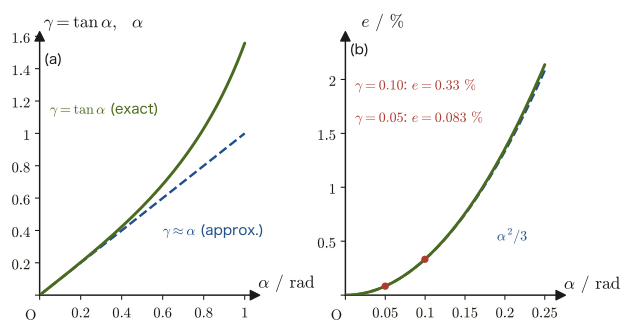
Math Tool: $\tan\alpha$ and the approximation $\tan\alpha\approx\alpha$ for small angles
$\tan\alpha$ (the tangent) is one of the trigonometric ratios learned in high school mathematics, defined for a right triangle as “the ratio of the opposite side to the adjacent side” (High School Mathematics, Section 3.1). The reason that $\gamma=\tan\alpha$ in Eq. \eqref{eq:18-shear-strain-def} is precisely that, in the right triangle of Figure 18.12 (height $l_0$, base $\lambda$), $\tan\alpha=(\text{opposite})/(\text{adjacent})=\lambda/l_0$. Moreover, since the angle $\alpha$ treated in mechanics of materials is extremely small (the “small-deformation assumption” of Section 18.1), if we replace $\tan\alpha$ by the first-order approximation of the Taylor expansion about $\alpha=0$ (University Mathematics, Section 4.1), the good approximation $\tan\alpha\approx\alpha$ ($\alpha$ being the value in radians, as measured by radian measure) holds. An angle measured in radians is the ratio of the arc length to the radius, a dimensionless quantity obtained by dividing a length by a length. It is in this sense that the shear strain $\gamma=\tan\alpha$, although it is an angle, can be treated as the dimensionless quantity called “strain.”
Example 18.11: Shear strain, comparing the exact angle with the approximation
A shear load is applied to the top face of a cubic rubber block of edge length $l_0=50\ \mathrm{mm}$, and the top face is displaced by $\lambda=5\ \mathrm{mm}$ relative to the bottom face. Find the shear strain $\gamma$. Also, compare the angle of displacement $\alpha$ found (a) exactly (using $\arctan$) with that found (b) using the small-angle approximation $\alpha\approx\gamma$ (the approximation that regards the value in radians directly as the angle), and discuss the difference between the two.
Solution. From Definition 18.9 (Eq. \eqref{eq:18-shear-strain-def}), we have
$$ \gamma=\frac{\lambda}{l_0}=\frac{5\ \mathrm{mm}}{50\ \mathrm{mm}}=0.10 $$(a) The exact angle is obtained from $\alpha=\arctan\gamma$, which is $\gamma=\tan\alpha$ solved for $\alpha$:
$$ \alpha_{\text{exact}}=\arctan(0.10)\approx0.09967\ \mathrm{rad}\ (\approx5.711^\circ) $$(b) In the small-angle approximation we simply set $\alpha\approx\gamma$, so
$$ \alpha_{\text{approx}}\approx\gamma=0.10\ \mathrm{rad}\ (\approx5.730^\circ) $$The relative error between the two is
$$ \frac{\abs{\alpha_{\text{exact}}-\alpha_{\text{approx}}}}{\alpha_{\text{exact}}}=\frac{\abs{0.09967-0.10000}}{0.09967}\approx0.33\ \% $$Thus, even for $\gamma=0.10$, a rather large shear strain by the standards of mechanics of materials, the error of the approximation remains only about $0.33\ \%$. The shear strain of actual metals and ceramics within the elastic range is often about $\gamma\sim10^{-3}$ or less, and for such a small $\gamma$ the error of the approximation $\alpha\approx\gamma$ is smaller still (Figure 18.13).
Finally, we define the strain that expresses how much the volume of the material as a whole changes.
Definition 18.10: Volumetric strain
When a body of volume $V$ is deformed by external forces and undergoes a volume change $\Delta V$, the value $\varepsilon_V$ obtained by dividing $\Delta V$ by the original volume $V$ is called the volumetric strain.
\begin{equation} \varepsilon_V\overset{\mathrm{def}}{=}\frac{\Delta V}{V} \label{eq:18-volumetric-strain-def} \end{equation}Derivation: Expressing the volumetric strain in terms of the longitudinal and transverse strains (first-order approximation)
Suppose that a rectangular block (edge lengths $l_x,l_y,l_z$) is deformed so that the strains in the directions of the respective edges (the fractional changes in the edge lengths) become $\varepsilon_x,\varepsilon_y,\varepsilon_z$. As in Eq. \eqref{eq:18-strain-def} of Definition 18.7, the edge lengths after the deformation can be written $l_x(1+\varepsilon_x)$, $l_y(1+\varepsilon_y)$, and $l_z(1+\varepsilon_z)$. The volume before the deformation is $V=l_xl_yl_z$, and the volume after the deformation is
$$ V+\Delta V=l_x(1+\varepsilon_x)\times l_y(1+\varepsilon_y)\times l_z(1+\varepsilon_z)=l_xl_yl_z(1+\varepsilon_x)(1+\varepsilon_y)(1+\varepsilon_z) $$Therefore, by the definition in Eq. \eqref{eq:18-volumetric-strain-def},
$$ \varepsilon_V=\frac{\Delta V}{V}=\frac{V(1+\varepsilon_x)(1+\varepsilon_y)(1+\varepsilon_z)-V}{V}=(1+\varepsilon_x)(1+\varepsilon_y)(1+\varepsilon_z)-1 $$Expanding the right-hand side, we obtain
$$ (1+\varepsilon_x)(1+\varepsilon_y)(1+\varepsilon_z)-1=\varepsilon_x+\varepsilon_y+\varepsilon_z+\underbrace{(\varepsilon_x\varepsilon_y+\varepsilon_y\varepsilon_z+\varepsilon_z\varepsilon_x)}_{\text{second-order infinitesimal}}+\underbrace{\varepsilon_x\varepsilon_y\varepsilon_z}_{\text{third-order infinitesimal}} $$By the “small-deformation assumption” of Section 18.1, $\varepsilon_x,\varepsilon_y,\varepsilon_z$ are all quantities very small compared with 1 (for example, of the order of $10^{-4}\text{–}10^{-3}$). Therefore the second- and third-order terms, which are products of them (for example, $\varepsilon_x\varepsilon_y\sim10^{-8}\text{–}10^{-6}$ in order of magnitude), are smaller by many orders of magnitude than the first-order terms $\varepsilon_x,\varepsilon_y,\varepsilon_z$ (of magnitude $\sim10^{-4}\text{–}10^{-3}$), and may be neglected. This is the same “first-order approximation” idea as the $\tan\alpha\approx\alpha$ used in the first half of Section 18.5 (neglecting the higher-order terms of the Taylor expansion; University Mathematics, Section 4.1). Neglecting infinitesimal quantities of second order and higher, we obtain the result
\begin{equation} \varepsilon_V\approx\varepsilon_x+\varepsilon_y+\varepsilon_z \label{eq:18-volumetric-strain-approx} \end{equation}that the volumetric strain can be approximated as the simple sum of the strains in the three directions.
Special case: uniaxial tension. When a bar is pulled in the axial direction (the $x$ direction), the strain in the $x$ direction, $\varepsilon_x=\varepsilon$, is the longitudinal strain, and the strains in the two perpendicular directions, $\varepsilon_y=\varepsilon_z=\varepsilon'$, are the transverse strain (only in uniaxial tension do the strains along the individual axes coincide with the longitudinal and transverse strains). Substituting $\varepsilon'=-\nu\varepsilon$ (Definition 18.8) into Eq. \eqref{eq:18-volumetric-strain-approx}, we obtain
\begin{equation} \varepsilon_V\approx\varepsilon+2\varepsilon'=\varepsilon(1-2\nu) \label{eq:18-uniaxial-vol} \end{equation}Therefore $\varepsilon_V=0$ (the volume does not change; the material is incompressible) only when $\nu=1/2$, and for ordinary materials with $\nu\lt1/2$ we have $\varepsilon_V\gt0$; that is, the volume increases slightly when the material is pulled. In an isotropic elastic body $\nu\gt1/2$ does not occur (because the bulk modulus $K=E/\{3(1-2\nu)\}$ must be positive; Section 19.3). Even for a negative Poisson's ratio, with which the material becomes thicker sideways (auxetic materials, the Application in Section 18.4), we have $1-2\nu\gt1$, so that $\varepsilon_V\gt0$. A problem that examines the volumetric strain in uniaxial tension in detail is Exercise 18.6.
∎
Example 18.12: First-order approximation of the volumetric strain
A rectangular block made of a material with Poisson's ratio $\nu=0.30$ is pulled in the $x$ direction, producing a strain $\varepsilon_x=2.0\times10^{-4}$ (elongation) in the $x$ direction and strains $\varepsilon_y=\varepsilon_z=-\nu\varepsilon_x=-0.6\times10^{-4}$ (contraction) in the $y,z$ directions, respectively. Calculate the volumetric strain $\varepsilon_V$ both (a) by the first-order approximation of Eq. \eqref{eq:18-volumetric-strain-approx} and (b) by the exact expression $\varepsilon_V=(1+\varepsilon_x)(1+\varepsilon_y)(1+\varepsilon_z)-1$, and compare the results.
Solution. (a) In the first-order approximation (Eq. \eqref{eq:18-volumetric-strain-approx}),
$$ \varepsilon_V\approx\varepsilon_x+\varepsilon_y+\varepsilon_z=2.0\times10^{-4}+(-0.6\times10^{-4})+(-0.6\times10^{-4})=0.8\times10^{-4} $$This agrees with $\varepsilon(1-2\nu)=2.0\times10^{-4}\times(1-0.6)=0.8\times10^{-4}$ from Eq. \eqref{eq:18-uniaxial-vol}. (b) With the exact expression,
$$ \varepsilon_V=(1+2.0\times10^{-4})(1-0.6\times10^{-4})^{2}-1\approx7.998\times10^{-5} $$The difference between the two is about $2\times10^{-8}$, and the relative error with respect to the value of the first-order approximation is only about $0.03\ \%$. Thus, under the small-deformation assumption, the first-order approximation (Eq. \eqref{eq:18-volumetric-strain-approx}) has sufficient accuracy for practical purposes. Also, since the elongation in the $x$ direction is larger than the total contraction in the $y,z$ directions, the volume increases slightly overall ($\varepsilon_V\gt0$).
Application: Volumetric strain and the compressibility of materials
The volumetric strain is a quantity used, for example, to estimate how much an object sunk in the deep sea is compressed by the water pressure, or how much a material in a sealed container swells under internal pressure. The constant of proportionality between the volumetric strain and the hydrostatic stress that causes it (a compressive stress that pushes with the same magnitude from every direction, as in water) is the bulk modulus $K$, which is defined in the next chapter (Chapter 19). Also, as confirmed in Eq. \eqref{eq:18-uniaxial-vol} and Exercise 18.6, for a material under a tensile load in one direction, the volumetric strain of an ordinary material with $\nu\lt1/2$ is $\varepsilon_V=\varepsilon(1-2\nu)\gt0$, and the volume increases slightly when it is pulled. This is because the effect of the lateral contraction cannot fully cancel the longitudinal elongation; only in the case $\nu=1/2$ (rubber, for example), where the two cancel exactly, does the volume not change.
18.6 Summary and Exercises
18.6.1 Summary
- Mechanics of materials regards real materials as homogeneous bodies (Definition 18.1) and isotropic bodies (Definition 18.2), and discusses them under seven basic assumptions: internal force (Definition 18.3), small deformation, elasticity (Definition 18.4), the principle of superposition (Law 18.1), and Saint-Venant's principle (Law 18.2) (Table 18.1).
- Loads (Definition 18.5) are classified into five types according to the manner of action (tension, compression, shear, torsion, and bending), into concentrated loads and distributed loads according to the manner of distribution, and into static loads and dynamic loads (impact loads and repeated loads) according to the manner of variation in time.
- Stress (Definition 18.6) is the internal force per unit area; there are the normal stress $\sigma=P/A$, perpendicular to the cross section, and the shear stress $\tau=Q/A$, parallel to the cross section. The internal force is found by the method of sections, and $A$ is the cross-sectional area before deformation (nominal stress, also called engineering stress). The unit is $\mathrm{Pa}=\mathrm{N/m^2}$. In engineering, $\mathrm{MPa}=\mathrm{N/mm^2}$ is commonly used, and for elastic moduli $\mathrm{GPa}=10^{3}\ \mathrm{MPa}$ is often used. Keep to the sign convention that tension is positive and compression is negative.
- The longitudinal strain $\varepsilon=\Delta l/l_0$ and the transverse strain $\varepsilon'=\Delta d/d_0$ (Definition 18.7) are dimensionless quantities. The ratio of their absolute values is Poisson's ratio $\nu=\abs{\varepsilon'/\varepsilon}$, and its reciprocal is Poisson's number $m=1/\nu$ (Definition 18.8).
- The shear strain is $\gamma=\lambda/l_0=\tan\alpha$ (Definition 18.9). For small angles, $\tan\alpha\approx\alpha$ (the first-order approximation of the Taylor expansion) holds.
- The volumetric strain $\varepsilon_V=\Delta V/V$ (Definition 18.10) can be approximated under small deformation as $\varepsilon_V\approx\varepsilon_x+\varepsilon_y+\varepsilon_z$ (a first-order approximation that neglects infinitesimal quantities of second order and higher). In uniaxial tension, $\varepsilon_V\approx\varepsilon(1-2\nu)$, and the volume remains unchanged only when $\nu=1/2$.
In the next chapter (Chapter 19), we study the proportional relation that connects the stress and strain defined in this chapter—Hooke's law—and define three elastic moduli: Young's modulus (the modulus of longitudinal elasticity) $E$, the shear modulus (the modulus of transverse elasticity) $G$, and the bulk modulus $K$.
18.6.2 Exercises
Exercise 18.1: Tensile stress in a bolt
A tensile load $P=8\ \mathrm{kN}$ acts on a bolt of diameter $d_0=12\ \mathrm{mm}$. Find the tensile stress $\sigma$ produced in this bolt, in $\mathrm{MPa}$, to three significant figures.
Hint: First find the cross-sectional area from $A_0=\pi(d_0/2)^2$ in $\mathrm{mm^2}$, and then compute $\sigma=P/A_0$ directly in $\mathrm{N/mm^2}=\mathrm{MPa}$ (the same procedure as in Example 18.6).
Exercise 18.2: Transverse strain in a steel bar
A longitudinal strain $\varepsilon=2.0\times10^{-4}$ (tensile) is produced in a steel bar with Poisson's ratio $\nu=0.30$. Find the resulting transverse strain $\varepsilon'$.
Hint: Use Definition 18.8 (Eq. \eqref{eq:18-poisson-def}), and note that when the longitudinal strain is positive (tension), the transverse strain is negative.
Exercise 18.3: Exact and approximate angles for the shear strain $\gamma=0.05$
When the shear strain is $\gamma=0.05$, find the angle of displacement $\alpha$ (a) exactly (using $\arctan$) and (b) using the small-angle approximation $\alpha\approx\gamma$. (c) Find the difference (relative error) between (a) and (b), compare it with the case of Example 18.11 ($\gamma=0.10$), and discuss which of the two approximations is better.
Hint: The relative error becomes smaller as $\gamma$ becomes smaller (refer to Figure 18.13, where the two curves approach each other the closer $\alpha$ is to 0).
Exercise 18.4: Which basic assumption tends to break down in porous materials?
Consider a metal foam (a metallic material with many pores inside). Of the basic assumptions (i)–(vii) in Section 18.1, which assumption is considered especially unlikely to hold for a metal foam? Explain together with the reason.
Hint: Compare the condition in Definition 18.1 (homogeneous body), “there are no defects or cavities inside,” with a metal foam full of pores. Also consider what happens if the sizes or the distribution of the pores are biased depending on direction.
Exercise 18.5: Saint-Venant's principle and the width of a member
When a concentrated load acts on the end of a flat plate of width $b$, how far from the point of application of the load, roughly, must one go for the stress distribution to be regarded as nearly uniform, according to Saint-Venant's principle? State a general rule of thumb using the width $b$. Also explain that the underlying idea is the same as in the case of the circular hole in Example 18.2 (a distance of two to three times the diameter from the center of the hole).
Hint: In Example 18.2, the disturbance of the stress became small at a distance several times “the size of the region over which the force producing the disturbance acts (the hole diameter $d$).” Here, what corresponds to the size of the region of action is the width $b$.
Exercise 18.6: Derivation of $\varepsilon_V\approx\varepsilon+2\varepsilon'$ and the meaning of Poisson's ratio $\nu=1/2$
Consider a bar that is subjected to a tensile load in one direction (the longitudinal direction) only. Let the longitudinal strain be $\varepsilon$ and the transverse strain (assumed to arise equally in each of the two mutually perpendicular transverse directions) be $\varepsilon'$. Using the idea of the first-order approximation of the volumetric strain in Section 18.5, show that $\varepsilon_V\approx\varepsilon+2\varepsilon'$. Further, substitute $\varepsilon'=-\nu\varepsilon$ (Definition 18.8) to express $\varepsilon_V$ in terms of $\varepsilon$ and $\nu$ alone, confirm that the volumetric strain is $0$ (no volume change; incompressible) when Poisson's ratio is $\nu=1/2$, and state its physical meaning. Also answer what the sign of $\varepsilon_V$ is when $\nu\lt1/2$ (does the volume increase or decrease when the bar is pulled?).
Hint: In Eq. \eqref{eq:18-volumetric-strain-approx} ($\varepsilon_V\approx\varepsilon_x+\varepsilon_y+\varepsilon_z$), let $\varepsilon_x=\varepsilon$ (the longitudinal direction) and $\varepsilon_y=\varepsilon_z=\varepsilon'$ (the two mutually perpendicular transverse directions).
Exercise 18.7: Shear stress in a bolt
Two overlapping plates are fastened by a single bolt of diameter $d=8\ \mathrm{mm}$ (the same configuration as in Figure 18.5), and a shear load $Q=5\ \mathrm{kN}$ acts on the bolt. (a) Find the shear stress $\tau$ produced on the shear plane of the bolt, in $\mathrm{MPa}$. (b) If the shear strength of the bolt material (the bolt fails when the shear stress reaches this value) is $300\ \mathrm{MPa}$, how many $\mathrm{kN}$ is the load $Q_{\max}$ at which the bolt fails?
Hint: The shear plane is a circle of diameter $d$. Use $\tau=Q/A$ (Eq. \eqref{eq:18-shear-stress-def}), and in (b) use it in the form $Q=\tau A$.
Exercise 18.8: Conversion of stress units
(a) Express $1.5\ \mathrm{GPa}$ in $\mathrm{MPa}$ and in $\mathrm{Pa}$. (b) Express the atmospheric pressure $101.325\ \mathrm{kPa}$ in $\mathrm{N/mm^2}$. (c) If a tensile stress of $120\ \mathrm{MPa}$ is produced in a bar of cross-sectional area $250\ \mathrm{mm^2}$, how many $\mathrm{kN}$ is the tensile load acting on the bar?
Hint: $1\ \mathrm{GPa}=10^{3}\ \mathrm{MPa}=10^{9}\ \mathrm{Pa}$ and $1\ \mathrm{MPa}=1\ \mathrm{N/mm^2}$. For (c), rewrite $\sigma=P/A$ as $P=\sigma A$ and compute with $\mathrm{N/mm^2}\times\mathrm{mm^2}=\mathrm N$.
18.6.3 References
- Yasuhide Mochizuki, Physics Notes: Mechanics of Materials (handwritten lecture notes, in Japanese). The source of this chapter.
- S. P. Timoshenko, D. H. Young, Elements of Strength of Materials, 5th ed., Van Nostrand, 1968.
- S. P. Timoshenko, J. N. Goodier, Theory of Elasticity, 3rd ed., McGraw-Hill, 1970. (Saint-Venant's principle and the stress around a circular hole (Kirsch's solution).)
- R. C. Hibbeler, Mechanics of Materials, Pearson.