Chapter 1Description of Motion — Position, Velocity, Acceleration, and Vectors
In high school physics, you have presumably described the motion of an object using numbers that carry only a magnitude—“speed” and “acceleration”—and memorized and used the formulas $v=v_0+at$, $x=x_0+v_0t+\frac12at^2$, and $v^2=v_0^2+2a(x-x_0)$. However, high school physics alone does not fully explain why these formulas hold, or how they should be rewritten when the motion takes place not along a single straight line but in a plane or in space, as when a ball is thrown obliquely upward. University mechanics begins by answering this “why” and this “how to rewrite.”
There are two key ideas. The first is to treat position, velocity, and acceleration as “quantities having magnitude and direction”—vectors. The second is to redefine velocity as “the rate of change of position with time” and acceleration as “the rate of change of velocity with time,” that is, as derivatives. Once we have these two tools, we see that the three formulas memorized in high school are nothing more than the result of integrating the acceleration twice under the condition that “the acceleration is constant.”
This chapter builds from scratch the words and tools needed to read Chapter 2 and beyond—the particle (point mass) model, the vector formulation of position, displacement, velocity, and acceleration, the SI system of units, and a preview of the inner product (dot product) and the cross product, which are used throughout mechanics. After finishing this chapter, you will be able to (1) compute the velocity and acceleration of any motion by differentiation, (2) derive the three high school formulas on your own, and (3) check equations using units and dimensions.
- Chapter 1 (this chapter) Description of motion—formulating position, velocity, and acceleration as vectors and rederiving the high school physics formulas.
- Chapter 2 Newton's laws of motion—the equation of motion $\bm F=\dd\bm p/\dd t$, conservation of momentum, torque (moment of force) and angular momentum.
- Chapter 3 Description of curvilinear motion—polar coordinates, and acceleration resolved along the tangential and normal directions.
- Chapter 4 Work and energy—the definition of work using the inner product, conservative forces and potential energy.
- Chapter 5 Projectile motion and circular motion—projectile motion with air resistance, centripetal acceleration.
- Chapter 6 Motion in polar coordinates and conic sections—trajectories as ellipses, parabolas, and hyperbolas.
- Chapter 7 Simple harmonic, damped, and forced oscillations—the mass on a spring and resonance.
- Chapter 8 Central forces and planetary motion—Kepler's laws and universal gravitation.
- Chapter 9 Moving reference frames and fictitious forces (inertial forces)—centrifugal and Coriolis forces.
- Chapter 10 Systems of particles and rigid bodies—motion of the center of mass, moment of inertia, and the rotational equation of motion.
- The particle model (a point whose size is ignored), and how to tell the situations in which it is valid from those in which it is not
- The definitions of the position vector $\bm r(t)$, the displacement vector $\Delta\bm r$, the velocity vector $\bm v=\dd\bm r/\dd t$, and the acceleration vector $\bm a=\dd^2\bm r/\dd t^2$ (including how to compute them as component-by-component derivatives), and the notation $\dot x,\ddot x$ for time derivatives
- The distinction between scalar and vector quantities, and how to use components, magnitudes, and the unit vectors $\bm e_x,\bm e_y,\bm e_z$
- The SI base units (m, kg, s, etc.) and derived units, SI prefixes and unit conversion, and the idea of dimensional analysis
- How to derive the three high school physics formulas $v=v_0+at$, $x=x_0+v_0t+\frac12at^2$, and $v^2=v_0^2+2a(x-x_0)$ by integrating twice the differential equation $\ddot x=a$, which expresses the condition that the acceleration is constant, and their application to free fall and vertical upward throw
- The meaning of the slope and the area in $x$-$t$ graphs and $v$-$t$ graphs (the geometric correspondence between differentiation and integration)
- A review of the inner and cross products, and a preview of the situations in mechanics in which the inner product appears as work and the cross product appears as torque and angular momentum
Related notes: This chapter supplements material not in the notes. Related notes: Yasuhide Mochizuki, Physics Notes: Mechanics (handwritten lecture notes, in Japanese).
1.1 The Particle Model
Balls, automobiles, the Earth—the “objects” we will treat in mechanics all have size and shape, and all have various kinds of internal structure. For example, when an automobile runs, its tires rotate, and its body tilts slightly or vibrates. Strictly speaking, to describe completely the motion of the object called an automobile, we would have to follow how every point of the body moves individually. However, if we are interested only in the overall path (the trajectory) of the motion “the automobile travels from Tokyo to Osaka,” the size of the body (a few meters) is far too small compared with the distance traveled (several hundred kilometers), and whichever point of the car we focus on, the differences in the trajectory can be almost entirely neglected. In such a case, an approximation that completely ignores the size and internal structure of the object and treats it as “a point that has mass but no size” becomes extremely effective.
Definition 1.1: Particle (point mass)
The model in which we ignore the size, shape, and internal structure of an object and regard its entire mass $m$ as concentrated at a single geometric point located at the object's center of mass (defined in Chapter 10) is called a particle (or point mass). The position of a particle (at a given time) is specified by just a single position vector $\bm r$ (introduced in Section 1.2), and the properties of the object are represented by the mass $m$ alone. Note that, in order to predict the motion, the velocity is needed in addition to the position (we will see this in Section 1.4 and Chapter 2).
Intuition: Conditions under which the particle approximation is a good approximation
Whether an object may be treated as a particle is not determined by whether the object itself is absolutely small. What should be compared is the ratio of (1) the size of the object itself (a representative length $L_{\text{obj}}$) to (2) the characteristic length $L_{\text{motion}}$ of the motion under consideration (the distance traveled, the radius of curvature of the trajectory, the size of the apparatus, and so on). If $L_{\text{obj}}/L_{\text{motion}}\ll1$ (the symbol $\ll$ means “much smaller than”), the shape of the trajectory hardly changes even if the object is represented by a single point somewhere, so the particle approximation is a good approximation. Conversely, if this ratio is close to 1, or if we are interested in the rotation or deformation of the object itself, the particle approximation cannot be used—the criterion is not “whether it is small” but “whether it can be neglected for the problem at hand.”
Example 1.1: Checking the validity of the particle approximation numerically
(a) Consider the orbital motion of the Earth. Taking the radius of the Earth as $R_\oplus\approx6.4\times10^{3}\ \mathrm{km}$ and the mean distance from the Sun (the orbital radius) as $R_{\text{orbit}}\approx1.5\times10^{8}\ \mathrm{km}$, find the ratio $R_\oplus/R_{\text{orbit}}$ and determine whether the particle approximation is a good approximation. (b) For a figure skater spinning with the arms extended to a radius $r\approx0.6\ \mathrm{m}$, form the same ratio, compare it with (a), and explain why the particle approximation cannot be used.
Solution. (a) Computing the ratio gives
$$ \frac{R_\oplus}{R_{\text{orbit}}}=\frac{6.4\times10^{3}\ \mathrm{km}}{1.5\times10^{8}\ \mathrm{km}}\approx4.3\times10^{-5} $$which is smaller than 1 by orders of magnitude (it is about 1/23,000). Therefore, in considering the Earth's orbit (a distance traveled of about 940 million km in one year), the size of the Earth itself (a diameter of about 13,000 km) may be neglected, and the particle approximation is an excellent approximation.
(b) For the skater's radius of rotation $r\approx0.6\ \mathrm{m}$, the representative size of the skater's own body, such as height and shoulder width, is also comparable ($0.3\sim1.7\ \mathrm{m}$ or so), so forming the ratio gives
$$ \frac{L_{\text{obj}}}{L_{\text{motion}}}\sim\frac{1\ \mathrm{m}}{0.6\ \mathrm{m}}\sim1 $$which is of the order of 1. Moreover, the very phenomenon that the skater spins faster when the arms are drawn in (the conservation of angular momentum, which we study in Chapter 2) depends on the positional relationships among the parts of the body—that is, on information that disappears if we squash the skater into a single particle. Therefore, in this problem the particle approximation cannot be used, and we must treat the positions and motions of the parts of the body (arms, torso, and so on) separately. That is, we treat the skater as a collection of many particles (a system of particles, Chapter 10). (If the shape can be regarded as unchanging, as in a state with the arms held fixed and extended, we could approximate the skater as a rigid body; but when the arms are drawn in, the shape changes, so we treat the whole process of spinning faster not as a rigid body but as a system of particles.)
Intuition: The three levels of models—particle, system of particles, and rigid body
In mechanics, there are roughly three levels of models for representing an object. (1) Particle—a single point with its size neglected (treated from this chapter on). (2) System of particles—a collection of many particles that exert forces on one another (it already makes an appearance in the conservation of momentum in Chapter 2). (3) Rigid body—a system of particles in which the distances between the particles are always kept constant (Chapter 10). The particle is the simplest of these three levels and serves as the starting-point model. If we first understand concepts such as position, velocity, acceleration, and force completely for a particle, which has just one element, then systems of particles and rigid bodies extend naturally as “the argument for a particle, summed over the number of elements.” This is why this chapter (and the subject of mechanics as a whole) begins with the particle.
1.2 Position Vector, Displacement, Velocity, and Acceleration
The first step in describing the motion of a particle is to prepare a coordinate system (with $x,y,z$ axes) whose origin $\mathrm O$ is fixed in space, and to represent the position of the particle at each time $t$ by an arrow from the origin to the particle—the position vector.
Definition 1.2: Position vector
The arrow drawn from the origin $\mathrm O$ to the position of the particle at time $t$ is called the position vector, and it is written in terms of its components as
$$ \bm r(t)=[\,x(t),\ y(t),\ z(t)\,] $$Here $x(t),y(t),z(t)$ are the $x,y,z$ coordinates of the particle expressed as functions of time $t$, and they are called the components of the position vector. When we consider only one-dimensional motion (along a straight line), we write $\bm r(t)=x(t)$, using just one component.
Caution: Bold vectors and arrow vectors
In this book, vector quantities are denoted in boldface (bold type), as in $\bm r,\bm v,\bm a,\bm F$. These refer to exactly the same quantities as the notation with arrows, $\vec r,\vec v,\vec a,\vec F$, used in high school textbooks and in handwritten blackboard work; only the convention for writing them differs. (The companion volume “University Mathematics” (AD 02), by contrast, uses the arrow notation $\vec y(t)$—it is common to use boldface in print and arrows in handwriting.) Whichever notation is used, please understand that it refers to the same thing: a quantity that has magnitude and direction. We make this remark only in this chapter; from the following chapters on, we use boldface throughout.
Math Tool: Scalars and vectors, components, magnitude, and unit vectors
There are two kinds of physical quantities. Quantities that are determined by a numerical value (and unit) alone, such as mass, time, temperature, and energy, are called scalars, and quantities that have both magnitude and direction, such as position, displacement, velocity, acceleration, and force, are called vectors. The numbers $a_x,a_y,a_z$ of a vector $\bm a=[a_x,a_y,a_z]$ are called its components, and by the Pythagorean theorem the magnitude (length) of $\bm a$ is
$$ \abs{\bm a}=\sqrt{a_x^2+a_y^2+a_z^2} $$(for a position vector, this is the distance from the origin to the particle, $\abs{\bm r}=\sqrt{x^2+y^2+z^2}$). The sum and difference of vectors and multiplication by a scalar $c$ are defined by calculating component by component: $\bm a\pm\bm b=[a_x\pm b_x,\ a_y\pm b_y,\ a_z\pm b_z]$, $c\,\bm a=[ca_x,\ ca_y,\ ca_z]$.
The coordinate axes are chosen so that, when a right-handed screw is turned from the $x$-axis toward the $y$-axis, the direction in which the screw advances is the positive direction of the $z$-axis (a right-handed system). The vectors of length 1 pointing in the positive direction of each axis,
$$ \bm e_x=[1,0,0],\qquad \bm e_y=[0,1,0],\qquad \bm e_z=[0,0,1] $$are called unit vectors, and with them the position vector can be written $\bm r=x\,\bm e_x+y\,\bm e_y+z\,\bm e_z=[x,\ y,\ z]$ (“$[x,y,z]$, the components listed in a row” and “a sum of unit vectors” are two ways of writing the same thing). For details, see University Mathematics, Section 15.1.
Suppose a particle moves from time $t_1$ to time $t_2$ ($t_2\gt t_1$). The displacement vector expresses how much, and in what direction, its position has changed during that time.
Definition 1.3: Displacement vector
We define the displacement vector from the position $\bm r(t_1)$ at time $t_1$ to the position $\bm r(t_2)$ at time $t_2$ as
$$ \Delta\bm r=\bm r(t_2)-\bm r(t_1) $$(vector subtraction is subtraction component by component). Note that the displacement vector does not depend on the shape of the path the particle actually followed; it is determined only by the starting point and the end point (even if the particle takes a detour along the way, $\Delta\bm r$ does not change).
Caution: Displacement and distance traveled, average velocity and average speed
The displacement $\Delta\bm r$ is a vector determined only by the starting point and the end point, whereas the distance traveled (path length) is a scalar obtained by adding up the lengths actually traveled along the path, and it depends on the shape of the path. In general $\abs{\Delta\bm r}\le$ (distance traveled), and equality holds only when the particle moves along a straight line without turning back. For example, in a motion that makes one full loop and returns to the starting place, $\Delta\bm r=\bm 0$, but the distance traveled is the length of one full loop.
The displacement divided by the elapsed time $\Delta t=t_2-t_1$ is called the average velocity $\bm v_{\text{avg}}=\Delta\bm r/\Delta t$ (a vector quantity). On the other hand, the distance traveled divided by $\Delta t$ is the average speed (a scalar quantity), and in general the two do not coincide.
Example 1.2: Displacement vector and average velocity
A particle is at the position $\bm r(t_1)=[1.0,\,2.0]\ \mathrm m$ at time $t_1=1.0\ \mathrm s$ and at the position $\bm r(t_2)=[4.0,\,6.0]\ \mathrm m$ at time $t_2=3.0\ \mathrm s$. (a) Find the displacement vector $\Delta\bm r$. (b) Find the average velocity $\bm v_{\text{avg}}=\Delta\bm r/\Delta t$ ($\Delta t=t_2-t_1$) over this interval.
Solution. (a) By Definition 1.3, subtracting component by component,
$$ \Delta\bm r=\bm r(t_2)-\bm r(t_1)=[4.0-1.0,\ 6.0-2.0]=[3.0,\ 4.0]\ \mathrm m $$(b) Since $\Delta t=t_2-t_1=3.0-1.0=2.0\ \mathrm s$, dividing each component of $\Delta\bm r$ by $\Delta t$ (a scalar) gives
$$ \bm v_{\text{avg}}=\frac{\Delta\bm r}{\Delta t}=\frac{[3.0,\,4.0]\ \mathrm m}{2.0\ \mathrm s}=[1.5,\ 2.0]\ \mathrm{m/s} $$Its magnitude is $\abs{\bm v_{\text{avg}}}=\sqrt{1.5^2+2.0^2}=\sqrt{6.25}=2.5\ \mathrm{m/s}$. What we have found here is only the “average over a 2-second interval,” and the particle did not necessarily move with this velocity throughout that time—to know the velocity at each instant, we need the differentiation introduced next.
The value of the average velocity $\Delta\bm r/\Delta t$ changes depending on how long a time interval $\Delta t$ we take. If we want to know the “velocity right now” at some instant, say at time $t$, we should consider the limit in which $\Delta t$ is brought arbitrarily close to 0—this is precisely the definition of the derivative (University Mathematics, Section 1.4), and in the case of vectors we likewise consider the same limit component by component (University Mathematics, Definition 17.1).
Definition 1.4: Velocity vector
We define the velocity vector $\bm v(t)$ of the position vector $\bm r(t)=[x(t),y(t),z(t)]$ by differentiating each component with respect to time $t$:
\begin{equation} \bm v(t)=\diff{\bm r}{t}=\left[\,\diff{x}{t},\ \diff{y}{t},\ \diff{z}{t}\,\right] \label{eq:1-velocity-def} \end{equation}Written with a limit, this is $\bm v(t)=\lim_{\Delta t\to0}\dfrac{\bm r(t+\Delta t)-\bm r(t)}{\Delta t}$, which is nothing other than the limit $\Delta t\to0$ of the average velocity in Example 1.2. The time derivatives of the components of the velocity vector can also be written $\bm v=[\dot x,\dot y,\dot z]$, using $\dot x\equiv\dd x/\dd t$ (read “x dot”; a notation in which a single dot placed above the letter denotes a time derivative). The dot notation is the one Newton used, and in physics it is used only for derivatives with respect to time (for derivatives with respect to position, we use $\dd/\dd x$ or $f'(x)$).
The direction of the average velocity $\Delta\bm r/\Delta t$ is the direction of the chord joining two points of the trajectory, and in the limit $\Delta t\to0$ the direction of the chord approaches the direction of the tangent to the trajectory. Therefore, the velocity vector points in the direction of the tangent to the trajectory, and its magnitude is equal to the speed $\abs{\bm v}$.
Similarly, the acceleration vector expresses how quickly the velocity is changing. We simply differentiate the velocity vector with respect to time once more.
Definition 1.5: Acceleration vector
We define the acceleration vector $\bm a(t)$ of the velocity vector $\bm v(t)$ as
\begin{equation} \bm a(t)=\diff{\bm v}{t}=\diff{}{t}\left(\diff{\bm r}{t}\right)=\frac{\dd^2\bm r}{\dd t^2}=[\,\ddot x,\ \ddot y,\ \ddot z\,] \label{eq:1-accel-def} \end{equation}Here $\ddot x\equiv\dd^2x/\dd t^2$ (read “x double dot”; the result of differentiating $x$ twice with respect to time $t$) is a notation in which two dots denote a second-order time derivative. The acceleration vector is the position vector differentiated twice with respect to time, and in a motion in which the velocity changes at a constant rate (motion with constant acceleration, which we will see later), $\bm a$ is a constant vector.
Why can we differentiate component by component?
There are two reasons why we may define the derivative of a vector by the operation of “differentiating each component separately, as a scalar-valued function.” First, vector subtraction and division by a scalar are both operations carried out component by component. The detailed verification is already given in University Mathematics, Section 17.1 (Definition 17.1 and, right after it, “Why do the two definitions agree?”), so here we use only the result. Second, when the position vector is expanded in unit vectors as $\bm r(t)=x(t)\,\bm e_x+y(t)\,\bm e_y+z(t)\,\bm e_z$, the vectors $\bm e_x,\bm e_y,\bm e_z$ are constant vectors that do not move as time passes, so in the differentiation they come out in front like coefficients, and
$$ \diff{\bm r}{t}=\dot x\,\bm e_x+\dot y\,\bm e_y+\dot z\,\bm e_z $$follows. Therefore, to differentiate a vector-valued function, it suffices to differentiate the three scalar-valued functions $x,y,z$ separately, using the differentiation formulas learned in high school mathematics. This is the most basic rule of calculation, and we use it in every part of mechanics from this chapter on.
However, this simple rule holds only when the basis vectors do not move. In coordinate systems that use unit vectors whose directions change with the position of the particle (such as the unit vectors $\bm e_r,\bm e_\theta$ of the polar coordinates studied in Chapter 3), the time derivatives of these unit vectors themselves enter as well, so component-by-component differentiation alone is no longer enough.
The velocity vector $\bm v$ and its magnitude $\abs{\bm v}$ both tend to be called “velocity” in everyday language, but physics distinguishes them. $\bm v$ is itself the vector quantity having magnitude and direction, whereas $\abs{\bm v}=\sqrt{\dot x^2+\dot y^2+\dot z^2}$ (the unit is $\mathrm{m/s}$ for both) is the scalar quantity obtained by discarding the information about direction and extracting only the magnitude; this is called the speed. Even if the speed is constant, as long as the direction keeps changing, the velocity vector $\bm v$ is changing from moment to moment, and therefore the acceleration $\bm a=\dd\bm v/\dd t$ is not $\bm 0$—for example, in a motion around a circle at constant speed (uniform circular motion), the speed $\abs{\bm v}$ is constant, but because the direction changes continuously, there is always an acceleration directed toward the center (we treat this rigorously in Chapter 3). Please note that “constant speed” does not mean “zero acceleration”; this is a typical pitfall that is easy to fall into even in high school physics. Indeed, differentiating the square of the speed, $\abs{\bm v}^2=v_x^2+v_y^2+v_z^2$, with respect to time gives $2(v_x\dot v_x+v_y\dot v_y+v_z\dot v_z)=2\,\bm v\cdot\bm a$ (the inner product $\bm v\cdot\bm a$ will be reviewed in Section 1.7). Therefore, if the speed is constant, $\bm v\cdot\bm a=0$; that is, the acceleration is perpendicular to the velocity (Exercise 1.4(c)). An acceleration that changes only the direction without changing the speed has only a component perpendicular to the velocity.
Example 1.3: Component-by-component differentiation of a position vector
The position vector of a particle is given as a function of time $t$ by $\bm r(t)=[\,t,\ t^2,\ \sin t\,]$ ($t$ is measured in seconds, and the components are numerical values measured in meters; the argument of $\sin t$ is an angle measured in radians, and this is the case of $\sin\omega t$ with $\omega=1\ \mathrm{rad/s}$). (a) Find the velocity vector $\bm v(t)$ and the acceleration vector $\bm a(t)$. (b) Find $\bm v(0)$ and $\bm a(0)$ at $t=0$.
Solution. (a) Following Definition 1.4, we differentiate each component separately with respect to $t$. From $x(t)=t$ we get $\dot x=1$, from $y(t)=t^2$ we get $\dot y=2t$, and from $z(t)=\sin t$ we get $\dot z=\cos t$ (the differentiation formula for trigonometric functions; this formula holds only when angles are measured in radians), so
$$ \bm v(t)=[\,1,\ 2t,\ \cos t\,]\ \mathrm{m/s} $$Differentiating once more, from $\ddot x=0$, $\ddot y=2$, $\ddot z=-\sin t$ we obtain
$$ \bm a(t)=[\,0,\ 2,\ -\sin t\,]\ \mathrm{m/s^2} $$(b) Substituting $t=0$, since $\cos0=1,\ \sin0=0$,
$$ \bm v(0)=[\,1,\ 0,\ 1\,]\ \mathrm{m/s},\qquad \bm a(0)=[\,0,\ 2,\ 0\,]\ \mathrm{m/s^2} $$Note that a motion like the one in this example, in which the acceleration changes with time $t$ (the $z$ component is $-\sin t$), is a more general case than the “motion with constant acceleration” treated in the following sections.
1.3 SI Base Units, Derived Units, and Dimensional Analysis
In the previous section we attached the units $\mathrm m$ (meter), $\mathrm{m/s}$, and $\mathrm{m/s^2}$ to position, velocity, and acceleration. Where do these units come from, and by what rules are they constructed? A physical quantity is always accompanied by a unit, and dropping the unit and computing with the numerical value alone is a source of serious errors (just as serious as getting the number of significant figures wrong). In this section we review the framework of the system of units used internationally in present-day science (the International System of Units, abbreviated SI), and the technique called “dimensional analysis,” which uses units as a weapon to check the correctness of the results of a calculation.
Definition 1.6: SI base units
In the SI, the unit of every physical quantity is expressed as a combination of the following seven base units: length: meter ($\mathrm m$); mass: kilogram ($\mathrm{kg}$); time: second ($\mathrm s$); electric current: ampere ($\mathrm A$); thermodynamic temperature: kelvin ($\mathrm K$); amount of substance: mole ($\mathrm{mol}$); luminous intensity: candela ($\mathrm{cd}$). In Part I (Mechanics) of this book, we use only three of these: length $[\mathrm m]$, mass $[\mathrm{kg}]$, and time $[\mathrm s]$.
Fun fact: How the base units are defined today
Formerly, the kilogram was defined by the very metal weight known as the “International Prototype of the Kilogram,” kept in France. However, because the mass of a physical object can change slightly over the years, the 2019 revision of the SI redefined all seven base units by fixing exactly the numerical values of specific physical constants (taking them as defined values)—for example, the second is defined by the frequency of the hyperfine transition of the cesium-133 atom, $\Delta\nu_{\mathrm{Cs}}=9\,192\,631\,770\ \mathrm{Hz}$ (exact, defined value), the meter by the speed of light $c=299\,792\,458\ \mathrm{m/s}$ (exact, defined value), and the kilogram by the Planck constant $h=6.626\,070\,15\times10^{-34}\ \mathrm{J\,s}$ (exact, defined value). In everyday calculations there is almost no need to be conscious of this difference, but it is an interesting fact that symbolizes the idea that “a unit is a convention decided by humans.”
A unit built by multiplying and dividing base units, like the unit of velocity $\mathrm{m/s}$ or the unit of acceleration $\mathrm{m/s^2}$, is called a derived unit. Derived units often used in mechanics include the newton, $\mathrm N=\mathrm{kg\,m/s^2}$, the unit of force (from Newton's equation of motion $F=ma$), and the joule, $\mathrm J=\mathrm{N\,m}=\mathrm{kg\,m^2/s^2}$, the unit of energy and work. Every derived unit can ultimately be rewritten as a product of powers of $\mathrm{m},\mathrm{kg},\mathrm s$.
In actual calculations we also often use units with an SI prefix attached, such as $\mathrm{km}$ and $\mathrm{cm}$ (Table 1.1). The base unit of mass, $\mathrm{kg}$, is the only base unit that contains a prefix (k); for example, $1\ \mathrm g=10^{-3}\ \mathrm{kg}$.
| Prefix | Symbol | Factor | Example |
|---|---|---|---|
| giga | $\mathrm G$ | $10^{9}$ | $1\ \mathrm{GHz}=10^{9}\ \mathrm{Hz}$ |
| mega | $\mathrm M$ | $10^{6}$ | $1\ \mathrm{MPa}=10^{6}\ \mathrm{Pa}$ |
| kilo | $\mathrm k$ | $10^{3}$ | $1\ \mathrm{km}=10^{3}\ \mathrm m$ |
| centi | $\mathrm c$ | $10^{-2}$ | $1\ \mathrm{cm}=10^{-2}\ \mathrm m$ |
| milli | $\mathrm m$ | $10^{-3}$ | $1\ \mathrm{mm}=10^{-3}\ \mathrm m$ |
| micro | $\mu$ | $10^{-6}$ | $1\ \mu\mathrm m=10^{-6}\ \mathrm m$ |
| nano | $\mathrm n$ | $10^{-9}$ | $1\ \mathrm{nm}=10^{-9}\ \mathrm m$ |
Unit conversion is carried out by multiplying and dividing by relations such as “$1\ \mathrm{km}=1000\ \mathrm m$, $1\ \mathrm h=3600\ \mathrm s$.” For example, since $1\ \mathrm{km/h}=\dfrac{1000\ \mathrm m}{3600\ \mathrm s}=\dfrac{1}{3.6}\ \mathrm{m/s}$, dividing a value in $\mathrm{km/h}$ by 3.6 gives the value in $\mathrm{m/s}$. When squaring a unit with a prefix, square the prefix too ($1\ \mathrm{km^2}=(10^{3}\ \mathrm m)^2=10^{6}\ \mathrm{m^2}$). Also, in the examples of this book, the number of digits in an answer is chosen to match the number of digits in the given values (in most cases, two significant figures).
Definition 1.7: Dimension
The “kind” of a quantity, which tells which of the base quantities length, mass, and time a given physical quantity contains and to what power, is called its dimension. Whether we measure in meters, kilometers, or feet, a length has the same “dimension of length”—a dimension does not depend on the choice of unit. Denoting the dimensions of length, mass, and time by the symbols $[\mathrm L],[\mathrm M],[\mathrm T]$, respectively, the dimension of velocity, for example, is $[\mathrm{L\,T^{-1}}]$, that of acceleration is $[\mathrm{L\,T^{-2}}]$, and that of force is $[\mathrm{M\,L\,T^{-2}}]$. The dimension $[\mathrm L]$ and the unit $[\mathrm m]$ are different things: $[\mathrm L]$ is a symbol expressing the kind “is a length,” whereas $\mathrm m$ is one of the concrete rulers for measuring length.
Law 1.1: Dimensional homogeneity
In a physically correct equation (or an expression whose terms are joined by addition and subtraction), the dimensions of both sides—and of all the terms joined as a sum—must agree. This is called dimensional homogeneity. Quantities of different dimensions cannot be added together or joined by an equals sign (for example, an expression like “length + time” has no physical meaning).
A quantity whose dimension is $[\mathrm{L^0M^0T^0}]$, that is, 1 (for example, angles in radians and ratios of two quantities of the same kind) is called a dimensionless quantity. The argument $x$ of functions such as $\sin x,\ \cos x,\ \exp x,\ \ln x$ must be dimensionless (for example, in $\sin\omega t$, $\omega t$ is dimensionless, so the dimension of $\omega$ is $[\mathrm{T^{-1}}]$).
Intuition: Dimensional analysis is a tool for finding calculation errors, and also a tool for guessing formulas
Dimensional homogeneity is used in two ways. First, by comparing the dimensions of both sides of an equation you have derived yourself, you can detect, with fairly high probability, mistakes in the course of the calculation (forgetting to multiply or divide by a factor in a term, and so on)—if the dimensions do not match, the equation is certainly wrong somewhere. Second, when you know only what variables a quantity depends on, but not the exact coefficient, you can sometimes guess the “form” of the formula from dimensions alone (Example 1.4(b)). Note, however, that dimensional analysis alone does not determine even a dimensionless coefficient such as $2\pi$.
Example 1.4: Dimensional analysis—checking and guessing
(a) Check the dimension of each term on the right-hand side of the high school physics formula $v^2=v_0^2+2a(x-x_0)$, and verify that it agrees with the dimension of the left-hand side. (b) Suppose we know that the period $T$ of a pendulum is determined only by the length $l$ of the pendulum and the magnitude $g$ of the gravitational acceleration (it does not depend on the mass). Assume the form $T=C\,l^{\alpha}g^{\beta}$ ($C$ is a dimensionless constant), and find the exponents $\alpha,\beta$ by dimensional analysis.
Solution. (a) The dimension of velocity is $[v]=[\mathrm{L\,T^{-1}}]$, so the dimension of the left-hand side $v^2$ is $[\mathrm{L^2\,T^{-2}}]$. The first term on the right-hand side, $v_0^2$, is likewise $[\mathrm{L^2\,T^{-2}}]$. The second term is the product of the dimension of acceleration, $[a]=[\mathrm{L\,T^{-2}}]$, and the dimension of length, $[x-x_0]=[\mathrm L]$, so $[2a(x-x_0)]=[\mathrm{L\,T^{-2}}]\times[\mathrm L]=[\mathrm{L^2\,T^{-2}}]$ (since $2$ is a dimensionless number, it does not affect the dimension). Every term on the left-hand and right-hand sides has the same dimension $[\mathrm{L^2\,T^{-2}}]$, so Law 1.1 is satisfied.
(b) The dimension of the period is $[T]=[\mathrm T]$, that of the length is $[l]=[\mathrm L]$, and that of the gravitational acceleration is $[g]=[\mathrm{L\,T^{-2}}]$. Comparing the dimensions of both sides of $T=C\,l^{\alpha}g^{\beta}$ gives
$$ [\mathrm T]=[\mathrm L]^{\alpha}\,[\mathrm{L\,T^{-2}}]^{\beta}=[\mathrm L]^{\alpha+\beta}\,[\mathrm T]^{-2\beta} $$Comparing the exponent of $[\mathrm L]$ and the exponent of $[\mathrm T]$ on the right-hand side with those on the left-hand side, respectively, we obtain the simultaneous equations
$$ \alpha+\beta=0\ (\mathrm L\text{ exponent: no }\mathrm L\text{ on the left-hand side, so }0),\qquad -2\beta=1\ (\mathrm T\text{ exponent}) $$Solving these gives $\beta=-\tfrac12$ and $\alpha=-\beta=\tfrac12$, so we find that the period must have the form
$$ T=C\sqrt{\frac{l}{g}} $$Note that if $T$ depended on the mass $m$, the dimension $[\mathrm M]$ would remain on the right-hand side and fail to agree with the left-hand side ($[\mathrm T]$), since $l,g$ do not contain $[\mathrm M]$; hence $m$ cannot enter. Actually solving the pendulum's equation of motion (treated in Chapter 7) shows that $C=2\pi$ when the amplitude is small, but that specific numerical value is not determined by dimensional analysis alone—dimensional analysis tells us only the form, namely “in what combination $l$ and $g$ come into play.”
1.4 Motion with Constant Acceleration in One Dimension — Deriving the Three High-School Physics Formulas
From here on, we consider the case of a particle moving along a single straight line (the $x$-axis) whose acceleration does not depend on time—motion with constant acceleration. If we let the acceleration be a constant $a$, then by Definition 1.5 the condition that the acceleration is constant is expressed by the differential equation
$$ \ddot x=a\quad(a\text{ is a constant}) $$This is merely an equation that writes down the condition “the acceleration is constant”; it is not Newton's equation of motion (Chapter 2). As we will learn in Chapter 2, if the force $F$ is constant, then the acceleration $a=F/m$ is also constant; for example, when only the gravitational force $F=-mg$ acts, we have $a=-g$.
This differential equation alone does not determine the motion—each time we integrate both sides a constant of integration appears, so integrating twice leaves two constants. We therefore determine the constants by giving the position $x_0=x(0)$ and the velocity $v_0=v(0)=\dot x(0)$ at time $t=0$ (the initial conditions). In high school physics you were probably given formulas such as $v=v_0+at$ out of the blue, but all of them can be derived simply by integrating this differential equation.
Derivation: Velocity and position when the acceleration is constant
(1) The equation for velocity. From the definition $\dot x=\dd x/\dd t$, the acceleration can also be written as $a=\dd v/\dd t$ ($v=\dot x$). Integrating both sides with respect to $t$ (an indefinite integral is the operation of finding a function that returns the original function when differentiated—an antiderivative—and each integration leaves a degree of freedom in the form of a constant $C$), we obtain
$$ \int\dd v=\int a\,\dd t \qquad\Longrightarrow\qquad v(t)=at+C_1 $$($a$ is a constant, so it can be taken outside the integral; $C_1$ is the constant of integration). Substituting $t=0$ gives $v(0)=C_1$, and since this must equal the initial velocity $v_0$, we have $C_1=v_0$. Therefore,
\begin{equation} v(t)=v_0+at \label{eq:1-v-of-t} \end{equation}(2) The equation for position. Eq. \eqref{eq:1-v-of-t} is also the first-order differential equation $\dd x/\dd t=v_0+at$, so we again integrate both sides with respect to $t$:
$$ \int\dd x=\int(v_0+at)\,\dd t \qquad\Longrightarrow\qquad x(t)=v_0t+\frac12at^2+C_2 $$Substituting $t=0$ gives $x(0)=C_2=x_0$, so
\begin{equation} x(t)=x_0+v_0t+\frac12at^2 \label{eq:1-x-of-t} \end{equation}(3) The equation not containing the time. Solving Eq. \eqref{eq:1-v-of-t} for $t$ gives $t=(v-v_0)/a$ ($a\neq0$). Substituting this into Eq. \eqref{eq:1-x-of-t} and simplifying, we obtain
$$ x-x_0=v_0\cdot\frac{v-v_0}{a}+\frac12a\left(\frac{v-v_0}{a}\right)^{\!2} =\frac{2v_0(v-v_0)+(v-v_0)^2}{2a} =\frac{(v-v_0)(v+v_0)}{2a}=\frac{v^2-v_0^2}{2a} $$(The second equality puts the terms over a common denominator; the third is the factorization $2v_0(v-v_0)+(v-v_0)^2=(v-v_0)\{2v_0+(v-v_0)\}=(v-v_0)(v+v_0)$; and the last uses the formula for the product of a sum and a difference, $(v-v_0)(v+v_0)=v^2-v_0^2$.) Multiplying both sides by $2a$, we find
\begin{equation} v^2=v_0^2+2a(x-x_0) \label{eq:1-v2-eq} \end{equation}∎
Theorem 1.1: The three constant-acceleration formulas
Suppose a particle moves along the $x$-axis with a constant acceleration $a$, and that $x(0)=x_0,\ \dot x(0)=v_0$ at time $t=0$. Then at any time $t$ the following three equations hold:
\begin{align} v(t)&=v_0+at \notag\\ x(t)&=x_0+v_0t+\frac12at^2 \notag\\ v^2&=v_0^2+2a(x-x_0) \notag \end{align}These are exactly the same equations that you memorized as formulas in high school physics, and, as we saw in this section, they are obtained simply by integrating the differential equation $\ddot x=a$ ($a$ constant) once and twice and eliminating the time $t$. The answer to the question “Why do these three equations hold?” is “Because they are the solution of the differential equation that expresses the condition of constant acceleration.”
Correspondence with high-school formulas
High school textbooks often write the three formulas in a slightly different way from this book. Let us check the correspondence.
- $v=v_0+at$: This is the same as Eq. \eqref{eq:1-v-of-t} of this book.
- $x=v_0t+\frac12at^2$: In high school, one often takes the starting point to be the origin ($x_0=0$), or uses $x$ to mean the “displacement from $t=0$,” $x-x_0$. The content is the same as Eq. \eqref{eq:1-x-of-t} of this book ($x-x_0=v_0t+\frac12at^2$).
- $v^2-v_0^2=2ax$: Likewise, this uses $x$ to mean the displacement $x-x_0$, and it has the same content as Eq. \eqref{eq:1-v2-eq}.
- $x-x_0=\dfrac{v_0+v}{2}\,t$ (“displacement = average of the initial and final velocities × time”): From Eq. \eqref{eq:1-v-of-t} we have $v_0+v=2v_0+at$, so $\dfrac{v_0+v}{2}\,t=v_0t+\dfrac12at^2$, which agrees with Eq. \eqref{eq:1-x-of-t}. In Section 1.6 we also derive it as the area of a trapezoid in the $v$-$t$ graph.
Also, in high school one fixes a positive direction and treats velocity and acceleration as signed numbers (this book does the same in one dimension). Treatment as vectors, as we will see in the next box, is just the same calculation carried out component by component.
Generalization to vectors—each of the three components independently obeys the same equations
Suppose a particle moves in a plane or in space and the acceleration vector $\bm a$ is a constant vector that does not depend on time (that is, a constant acceleration whose magnitude and direction do not change). Then, by the guideline “differentiate a vector component by component” in Definitions 1.4 and 1.5 (Section 1.2), the three equations of Theorem 1.1 hold independently for each of the components $x,y,z$. For the velocity and the position, for example, they can be collected into the vector equations
$$ \bm v(t)=\bm v_0+\bm a\,t,\qquad \bm r(t)=\bm r_0+\bm v_0t+\frac12\bm a\,t^2 $$which look just like the one-dimensional equations ($\bm v_0=\bm v(0)$, $\bm r_0=\bm r(0)$). “One vector equation” is merely a way of writing, in a single equation, the fact that “one equation of the same form holds for each component (two equations for two dimensions, three for three dimensions)”; when we actually compute numerical values, we still just apply Theorem 1.1 component by component. The equation with the time $t$ eliminated can also be collected into vector form. From $\bm v=\bm v_0+\bm a\,t$ and $\bm r-\bm r_0=\bm v_0t+\frac12\bm a\,t^2$, using the inner product (the sum of the products of the components, which we review in Section 1.7), we get
$$ \abs{\bm v}^2-\abs{\bm v_0}^2=(\bm v_0+\bm a\,t)\cdot(\bm v_0+\bm a\,t)-\bm v_0\cdot\bm v_0 =2\,\bm v_0\cdot\bm a\,t+\abs{\bm a}^2t^2 =2\,\bm a\cdot\left(\bm v_0t+\frac12\bm a\,t^2\right) $$and therefore the relation
$$ \abs{\bm v}^2=\abs{\bm v_0}^2+2\,\bm a\cdot(\bm r-\bm r_0) $$holds. (This is also what one obtains by adding up, over $x,y,z$, the component-wise equations such as $v_x^2=v_{0x}^2+2a_x(x-x_0)$.) Multiplying both sides of this equation by $m/2$ and using $m\bm a=\bm F$, which we will learn in Chapter 2, we obtain $\frac12m\abs{\bm v}^2-\frac12m\abs{\bm v_0}^2=\bm F\cdot(\bm r-\bm r_0)$. This is the prototype of the “relation between work and energy” that we will learn in Chapter 4. Note also that, for vectors as well, the integration that finds the position from the velocity is an integration component by component, as has been verified in University Mathematics, Section 17.3.
Example 1.5: Braking distance of a car that applies its brakes
A car traveling at 72 km/h applies its brakes and comes to a stop with a constant deceleration of magnitude $5.0\ \mathrm{m/s^2}$. Find the distance traveled until it stops (the braking distance).
Solution. First, make the units consistent. Converting 72 km/h to meters per second, $v_0=72\ \mathrm{km/h}=72\times\dfrac{1000\ \mathrm m}{3600\ \mathrm s}=20\ \mathrm{m/s}$. Taking the direction of travel as positive, since the car is decelerating the acceleration is $a=-5.0\ \mathrm{m/s^2}$ (magnitude 5.0, direction opposite to the direction of travel). The velocity at the moment of stopping is $v=0$, so using the third equation of Theorem 1.1, Eq. \eqref{eq:1-v2-eq} (a convenient feature of this equation is that the distance is obtained directly without going through $t$), we have
$$ 0^2=20^2+2\times(-5.0)\times(x-x_0) \qquad\Longrightarrow\qquad x-x_0=\frac{-20^2}{2\times(-5.0)}=\frac{-400}{-10}=40\ \mathrm m $$The braking distance is $40\ \mathrm m$. Dimensional check: the right-hand side is $\mathrm{(m/s)^2/(m/s^2)}=\mathrm{m^2/s^2}\times\mathrm{s^2/m}=\mathrm m$, which agrees with the unit of the left-hand side (a distance).
Note that this calculation is valid only up to the time $t=v_0/\abs{a}=20/5.0=4.0\ \mathrm s$ at which $v=0$ (if we continued to use the equations beyond that time, the car would move backward). Moreover, the actual stopping distance also includes the reaction distance: during the reaction time between the driver noticing the danger and stepping on the brake (for example $0.75\ \mathrm s$), the car still travels at $20\ \mathrm{m/s}$, which adds $20\times0.75=15\ \mathrm m$, so the total distance until the car stops is $40+15=55\ \mathrm m$.
Example 1.6: Constant-acceleration motion in vector form
A particle moves under a constant acceleration vector $\bm a=[0,\,-9.8]\ \mathrm{m/s^2}$ (the acceleration of free fall due to gravity, with the $y$-axis taken vertically upward). If the position and velocity at time $t=0$ are $\bm r_0=[0,\,10]\ \mathrm m$ and $\bm v_0=[5.0,\,0]\ \mathrm{m/s}$, find the position vector $\bm r(2.0)$ and the velocity vector $\bm v(2.0)$ at $t=2.0\ \mathrm s$.
Solution. By the “Generalization to vectors” just above, we can simply apply Theorem 1.1 as it stands to each of the components $x,y$.
$x$-component ($a_x=0$): $x(t)=0+5.0t+\dfrac12\times0\times t^2=5.0t$, $v_x(t)=5.0+0\times t=5.0\ \mathrm{m/s}$ (constant).
$y$-component ($a_y=-9.8\ \mathrm{m/s^2}$): $y(t)=10+0\times t+\dfrac12\times(-9.8)\times t^2=10-4.9t^2$, $v_y(t)=0+(-9.8)t=-9.8t$.
Substituting $t=2.0\ \mathrm s$, we obtain
$$ x(2.0)=5.0\times2.0=10\ \mathrm m,\qquad y(2.0)=10-4.9\times2.0^2=10-19.6=-9.6\ \mathrm m $$ $$ v_x(2.0)=5.0\ \mathrm{m/s},\qquad v_y(2.0)=-9.8\times2.0=-19.6\ \mathrm{m/s} $$That is, $\bm r(2.0)=[10,\,-9.6]\ \mathrm m$ and $\bm v(2.0)=[5.0,\,-19.6]\ \mathrm{m/s}$. If we take $y=0$ to be ground level, the time at which $y(t)=10-4.9t^2=0$ is $t=\sqrt{10/4.9}\approx1.4\ \mathrm s$, so these equations describe motion above the ground only in the range $0\le t\le1.4\ \mathrm s$. The value $y=-9.6\ \mathrm m$, which is negative at $t=2.0\ \mathrm s$, is the value for the case where there is no ground and the particle simply keeps falling (for example, if it was thrown from the top of a cliff); here, as practice in evaluating the equations, we do not consider a collision with the ground. For reference, at $t=1.0\ \mathrm s$, when the particle is still in the air, $\bm r(1.0)=[5.0,\,5.1]\ \mathrm m$ and $\bm v(1.0)=[5.0,\,-9.8]\ \mathrm{m/s}$ (the full treatment of this kind of motion, which also has an initial velocity in the horizontal direction, including air resistance, is the projectile motion of Chapter 5).
Example 1.7: Position and velocity of a particle thrown obliquely upward
A particle is thrown from the point $\bm r_0=[0,\,0]$ on the ground (the $x$-axis is horizontal and the $y$-axis is vertically upward) with an initial speed of $20\ \mathrm{m/s}$ and an elevation angle (the angle measured upward from the horizontal plane) of $30^\circ$. Neglect air resistance and take the acceleration to be $\bm a=[0,\,-9.8]\ \mathrm{m/s^2}$. Find the position vector $\bm r$ and the velocity vector $\bm v$ at $t=1.0\ \mathrm s$.
Solution. First, we resolve the initial velocity vector into components. Its magnitude is $20\ \mathrm{m/s}$ and it points $30^\circ$ above the horizontal, so from $\cos30^\circ=\sqrt3/2\approx0.866$ and $\sin30^\circ=1/2$ we have
$$ \bm v_0=[\,20\cos30^\circ,\ 20\sin30^\circ\,]=[\,17.3,\ 10\,]\ \mathrm{m/s} $$We apply Theorem 1.1 to each component. $x$-component ($a_x=0$): $x(t)=17.3\,t$, $v_x(t)=17.3$. $y$-component ($a_y=-9.8$): $y(t)=10t-4.9t^2$, $v_y(t)=10-9.8t$. Substituting $t=1.0\ \mathrm s$, we obtain
$$ x(1.0)=17.3\ \mathrm m,\qquad y(1.0)=10\times1.0-4.9\times1.0^2=5.1\ \mathrm m $$ $$ v_x(1.0)=17.3\ \mathrm{m/s},\qquad v_y(1.0)=10-9.8\times1.0=0.2\ \mathrm{m/s} $$That is, $\bm r(1.0)=[17.3,\ 5.1]\ \mathrm m$ and $\bm v(1.0)=[17.3,\ 0.2]\ \mathrm{m/s}$. The reason $v_y$ is almost 0 is that the highest point, where the $y$-component of the velocity becomes 0, is reached at $t=10/9.8\approx1.02\ \mathrm s$, and $t=1.0\ \mathrm s$ is just before that.
Example 1.8: An electron accelerated in an electric field—constant-acceleration motion not due to gravity
An electron at rest in a vacuum (mass $m_{\mathrm e}=9.109\times10^{-31}\ \mathrm{kg}$, magnitude of charge $e=1.602\times10^{-19}\ \mathrm C$) starts to move under a force $F=eE$ of constant direction and magnitude due to a uniform electric field $E=1.0\times10^{3}\ \mathrm{V/m}$. (a) Find the magnitude $a$ of the acceleration and compare it with $g=9.8\ \mathrm{m/s^2}$. (b) Find the speed of the electron after it has traveled $1.0\ \mathrm{cm}$.
Solution. (a) From the relation between force and acceleration, $ma=F$ (to be learned in Chapter 2; here we use only the result), we have $a=F/m_{\mathrm e}=eE/m_{\mathrm e}$, so
$$ a=\frac{1.602\times10^{-19}\ \mathrm C\times1.0\times10^{3}\ \mathrm{V/m}}{9.109\times10^{-31}\ \mathrm{kg}}=1.76\times10^{14}\ \mathrm{m/s^2} $$(The unit is $\mathrm{C\,V/(m\,kg)}=\mathrm{J/(m\,kg)}=\mathrm{N/kg}=\mathrm{m/s^2}$, which agrees with the unit of acceleration.) This is $1.76\times10^{14}/9.8\approx1.8\times10^{13}$ times $g$. The gravitational force acting on the electron, $m_{\mathrm e}g\approx8.9\times10^{-30}\ \mathrm N$, is smaller than the electric force $eE=1.6\times10^{-16}\ \mathrm N$ by many orders of magnitude, so it can be neglected.
(b) The acceleration is constant and the initial velocity is $v_0=0$, so from the third equation of Theorem 1.1, Eq. \eqref{eq:1-v2-eq}, we have $v^2=2a(x-x_0)$. Substituting $x-x_0=1.0\ \mathrm{cm}=1.0\times10^{-2}\ \mathrm m$, we obtain
$$ v=\sqrt{2\times1.76\times10^{14}\ \mathrm{m/s^2}\times1.0\times10^{-2}\ \mathrm m}=\sqrt{3.5\times10^{12}}\ \mathrm{m/s}=1.9\times10^{6}\ \mathrm{m/s} $$(This is about 0.6% of the speed of light.) Thus, motion with constant acceleration is not limited to the case of gravity; whenever a constant force acts, it can be treated with the same equations. Estimates for devices that accelerate electrons in an electric field (cathode-ray tubes (Braun tubes), the electron guns of electron microscopes, and so on) are extensions of this calculation.
1.5 Free Fall and Vertical Upward Throw
The most familiar example of motion with constant acceleration is vertical (up-and-down) motion under the Earth's gravity. As long as air resistance can be neglected, every object near the Earth's surface, regardless of its mass, is accelerated vertically downward with the same magnitude of acceleration—the gravitational acceleration $g\approx9.8\ \mathrm{m/s^2}$. The value of $g$ varies slightly with latitude and altitude (roughly $9.78\sim9.83\ \mathrm{m/s^2}$; the internationally defined standard value is $9.80665\ \mathrm{m/s^2}$), but in this book we use $g=9.8\ \mathrm{m/s^2}$. The acceleration is the same regardless of mass because gravity is proportional to mass ($F=mg$), so that $m$ cancels from both sides of the equation of motion $ma=mg$, which we study in Chapter 2. This is a fact that Galileo Galilei discovered experimentally, and it was an important step in the history of mechanics, overturning the earlier intuitive idea that “heavier objects fall faster” (said to go back to Aristotle). (He is said to have confirmed it with experiments using balls rolling down inclines, and the anecdote that he dropped objects from the top of a tower is also told, but there are various views about the details as historical fact.)
Caution: Direction of the coordinate axis and the sign of $g$
When we treat vertical motion as one-dimensional motion with constant acceleration, we must first decide which direction of the $y$-axis is positive, and then keep to that convention consistently. In this book, unless stated otherwise, we take vertically upward as positive. Under this convention the acceleration due to gravity always acts downward (in the negative direction), so we write $a=-g$ (where $g=9.8\ \mathrm{m/s^2}\gt0$ is the magnitude). (Some textbooks take downward as positive and write $a=+g$, but the physical phenomenon itself does not change. To avoid confusing the meaning of the signs, make it a habit to always check for yourself, before starting a calculation, which direction you have taken as positive.)
Below, we denote the vertical coordinate by $y$. Theorem 1.1 can be used as it is if we replace $x,x_0$ by $y,y_0$ and $a$ by $-g$.
Free fall is the case in which an object is dropped with initial velocity 0 (released gently from the hand). Setting $v_0=0,\ a=-g$ in Theorem 1.1, we obtain
\begin{equation} v(t)=-gt,\qquad y(t)=y_0-\frac12gt^2 \label{eq:1-freefall} \end{equation}Thus the speed $\abs{v(t)}=gt$ increases in proportion to time, and the distance fallen $y_0-y(t)=\frac12gt^2$ increases in proportion to the square of the time.
Example 1.9: Free fall
A pebble is dropped gently (initial velocity 0) from the roof of a building of height $44.1\ \mathrm m$. Find the time it takes for the pebble to reach the ground and its speed just before it reaches the ground. Take $g=9.8\ \mathrm{m/s^2}$ and neglect air resistance.
Solution. Take the ground as the origin ($y=0$) and vertically upward as positive. Then the roof is at $y_0=44.1\ \mathrm m$, and the initial velocity is $v_0=0$. From Eq. \eqref{eq:1-freefall}, $y(t)=44.1-4.9t^2$. The pebble reaches the ground when $y(t)=0$, so
$$ 44.1-4.9t^2=0 \qquad\Longrightarrow\qquad t^2=\frac{44.1}{4.9}=9.0 \qquad\Longrightarrow\qquad t=3.0\ \mathrm s $$(we choose the solution with $t\gt0$). The velocity at this instant is, from Eq. \eqref{eq:1-freefall}, $v(3.0)=-9.8\times3.0=-29.4\ \mathrm{m/s}$ (the negative sign indicates downward), and the speed is $\abs{v}=29.4\ \mathrm{m/s}$ (about $106\ \mathrm{km/h}$ when converted to kilometers per hour).
A vertical upward throw (also called vertical projectile motion) is the case in which an object is thrown upward by giving it an initial velocity $v_0\gt0$ (upward). The acceleration itself is the same $a=-g$ as in free fall; the only difference is the initial velocity. By Theorem 1.1, the velocity and position are in general given by
$$ v(t)=v_0-gt,\qquad y(t)=y_0+v_0t-\frac12gt^2 $$The object decelerates as it rises, momentarily has velocity 0 at the highest point, and then reverses direction and begins to fall (before and after the highest point, the equation for the position traces a left-right symmetric parabola).
Example 1.10: Vertical upward throw—height of the highest point and time of flight
A ball is thrown straight up from the ground ($y_0=0$) with initial velocity $v_0=19.6\ \mathrm{m/s}$. (a) Find the height of the highest point. (b) Find the time it takes for the ball to return to the ground (the time of flight). Take $g=9.8\ \mathrm{m/s^2}$.
Solution. (a) At the highest point the ball is at rest for just an instant (the moment at which it rises no further and has not yet begun to fall), so $v=0$. Using the third equation of Theorem 1.1, Eq. \eqref{eq:1-v2-eq} ($x\to y$, $a=-g$, $x_0\to y_0=0$), we can find the height directly without going through $t$:
$$ 0^2=v_0^2+2(-g)(y_{\max}-0) \qquad\Longrightarrow\qquad y_{\max}=\frac{v_0^2}{2g}=\frac{19.6^2}{2\times9.8}=\frac{384.16}{19.6}=19.6\ \mathrm m $$(b) The ball returns to the ground when $y(t)=0$ ($t\gt0$). Since $y(t)=v_0t-\frac12gt^2=t\left(v_0-\frac12gt\right)$, $y(t)=0$ holds only at $t=0$ (the instant of departure) or when $v_0-\frac12gt=0$, that is, at the time
$$ t=\frac{2v_0}{g}=\frac{2\times19.6}{9.8}=4.0\ \mathrm s $$The time of flight is $4.0\ \mathrm s$, which is exactly twice the “time to reach the highest point,” $t_{\text{top}}=v_0/g=2.0\ \mathrm s$—this expresses a symmetry of the motion: the time taken to rise equals the time taken to fall.
Application: Situations in which the ideas of free fall and upward throws come into play
The equations for free fall and vertical upward throw hold exactly only in idealized situations (without air resistance), but over short times and at low altitudes they are good approximations to real phenomena. They are basic models that are also used in engineering and safety management—for example, the trajectory of a baseball or a basketball, estimating the time of fall when an elevator cable breaks, and calculations at construction sites that assess the danger zone from the time a falling object takes to reach the ground. For objects such as a scrap of paper or a feather, for which the effect of air resistance cannot be neglected, the equations of this section are not good approximations—a more realistic projectile motion that takes air resistance into account is treated in Chapter 5.
1.6 $x$-$t$ Graphs and $v$-$t$ Graphs — Slope and Area
So far we have described motion with equations, but if we draw position and velocity as functions of time in a graph, we can read off the nature of the motion at a glance. A graph with time $t$ on the horizontal axis and position $x$ (or $y$) on the vertical axis is called an $x$-$t$ graph, and a graph with velocity on the vertical axis is called a $v$-$t$ graph. The “slope” and the “area” of these graphs express the geometric meaning of the very calculations of differentiation and integration.
Intuition: Slope is differentiation, area is integration
Slope. By Definition 1.4, $v=\dot x=\dd x/\dd t$, so the slope of the tangent to the $x$-$t$ graph at a given time equals the velocity $v$ at that instant. Similarly, since $a=\dot v$, the slope of the tangent to the $v$-$t$ graph equals the acceleration $a$ at that instant. The more steeply the graph rises to the right, the larger the positive value of the velocity (or acceleration); if the graph is horizontal, the velocity (acceleration) is 0; and if the graph falls to the right, the value is negative.
Area. Conversely, the area of the region enclosed by the graph and the $t$-axis in a $v$-$t$ graph between time $t_1$ and time $t_2$ (the part below the $t$-axis is counted with a sign, that is, as a negative area) is equal to the displacement during that interval, namely
$$ x(t_2)-x(t_1)=\int_{t_1}^{t_2}v(t)\,\dd t $$This is a restatement, in terms of the area of a graph, of the relation that integrating the velocity with respect to time gives the displacement (the definition of the definite integral by Riemann sums in University Mathematics, Section 5.3, and the fundamental theorem of calculus). Similarly, the area of an $a$-$t$ graph is equal to the change in velocity, $v(t_2)-v(t_1)=\int_{t_1}^{t_2}a(t)\,\dd t$. This correspondence, “slope = differentiation” and “area = integration,” is a graphical expression of the fact that the three quantities $x,v,a$ are connected to one another by the relations of differentiation and integration, and it is a basic principle that we hope you will always keep in mind when you read graphs in mechanics.
Derivation: The $v$-$t$ graph and $x$-$t$ graph of motion with constant acceleration
The $v$-$t$ graph representing $v(t)=v_0+at$ for motion with constant acceleration is a straight line with intercept $v_0$ and slope $a$. The area from time $0$ to $t$ is that of a trapezoid with upper base $v_0$, lower base $v=v_0+at$, and height $t$, so by the formula for the area of a trapezoid we have
$$ x-x_0=\frac12(v_0+v)\,t=\frac12(2v_0+at)\,t=v_0t+\frac12at^2 $$Thus Eq. \eqref{eq:1-x-of-t} is obtained without using integration (the intermediate expression $x-x_0=\frac{v_0+v}{2}\,t$ is the form of the “average velocity” that is also used in high school). On the other hand, in the $x$-$t$ graph the slope is $v$, and $v$ changes at the constant rate $a$, so the graph is a parabola. When $a\gt0$ ($\ddot x\gt0$) it is concave up, when $a\lt0$ it is concave down, and if $a=0$ it is a straight line (uniform motion). That is, the way the $x$-$t$ graph curves indicates the sign of the acceleration.
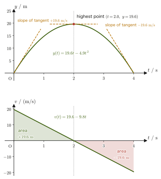
Example 1.11: Finding the displacement from the area of the $v$-$t$ graph
For Example 1.10 (the ball thrown straight up with $y_0=0$, $v_0=19.6\ \mathrm{m/s}$, $a=-9.8\ \mathrm{m/s^2}$): (a) Find the displacement from $t=0$ to $t=2.0\ \mathrm s$ as the area of the $v$-$t$ graph. (b) Find the displacement from $t=2.0$ to $t=4.0\ \mathrm s$ in the same way, and explain the meaning of the sign. (c) Find the displacement and the distance traveled over the whole interval $0\le t\le4.0\ \mathrm s$, and explain the difference between them.
Solution. Since $v(t)=19.6-9.8t$ is a linear function (a straight line) of $t$, the $v$-$t$ graph is a straight line, and the “area” of each interval can be calculated as the area of a triangle.
(a) At $t=0$, $v(0)=19.6\ \mathrm{m/s}$, and at $t=2.0$, $v(2.0)=19.6-9.8\times2.0=0$. In this interval the graph lies above the $t$-axis (the velocity is always positive; the ball is still rising), forming a right triangle with height $19.6$ and base $2.0$. The area (= the displacement) is
$$ \Delta y=\frac12\times2.0\times19.6=19.6\ \mathrm m $$This agrees exactly with the height of the highest point, $y_{\max}=19.6\ \mathrm m$, found in Example 1.10(a)—the distance risen up to the highest point is precisely the area from $t=0$ to $2.0\ \mathrm s$.
(b) At $t=2.0$, $v=0$, and at $t=4.0$, $v(4.0)=19.6-9.8\times4.0=-19.6\ \mathrm{m/s}$. In this interval the graph lies below the $t$-axis (the velocity is negative; the ball is descending), and a triangle with base $2.0$ and height $19.6$ is formed below the $t$-axis. The signed area (= the displacement) is
$$ \Delta y=-\frac12\times2.0\times19.6=-19.6\ \mathrm m $$The negative sign indicates that in this interval the ball was displaced by $19.6\ \mathrm m$ in the negative direction of the $y$-axis (downward)—that is, it fell from the highest point to the height of the starting point (the ground, $y=0$). That the magnitudes of the areas in (a) and (b) are equal confirms once more, in the form of areas on the graph, the symmetry of the motion seen in Example 1.10: the distance covered in rising equals the distance covered in falling.
(c) The total displacement is the sum of the signed areas in (a) and (b), $19.6+(-19.6)=0$, so the ball has returned to its starting point. On the other hand, the distance actually traveled, obtained by adding the areas enclosed by the graph and the $t$-axis without signs ($\int\abs{v}\,\dd t$), is $19.6+19.6=39.2\ \mathrm m$. The displacement (a vector, signed) and the distance traveled (a scalar) are different quantities, and what the signed area of the $v$-$t$ graph represents is the displacement.
1.7 A Preview of Inner and Cross Products — Where They Appear in Mechanics
So far, our vector calculations have required only addition, subtraction, and scalar multiplication (multiplication by a constant). Mechanics, however, involves two kinds of “products of vectors” that build a new quantity from two vectors—the inner product, whose result is a scalar, and the cross product, whose result is a vector. Both are studied in detail in University Mathematics, Chapter 15; in this section we briefly review their definitions and preview where they will be used in mechanics.
Math Tool: Inner product (review)
The inner product (also called the scalar product or dot product) of two vectors $\bm a=[a_x,a_y,a_z]$ and $\bm b=[b_x,b_y,b_z]$ is defined as the sum of the products of their components
$$ \bm a\cdot\bm b=a_xb_x+a_yb_y+a_zb_z $$and, if $\theta$ denotes the angle between the two vectors, it has the geometric meaning $\bm a\cdot\bm b=\abs{\bm a}\abs{\bm b}\cos\theta$ (for the detailed definition and proof, see University Mathematics, Section 15.2). The result of the inner product is a scalar (a real number) with no direction, and when $\theta=90°$ (the vectors are orthogonal), $\cos\theta=0$ and the inner product is 0. Geometrically, $\bm a\cdot\bm b$ can be understood as the product of “the length of the orthogonal projection of $\bm b$ onto the direction of $\bm a$” and $\abs{\bm a}$. In particular, since $\bm a\cdot\bm a=\abs{\bm a}^2$, the square of the speed can be written $\abs{\bm v}^2=\bm v\cdot\bm v$.
Math Tool: Cross product (review)
The cross product (also called the vector product) $\bm a\times\bm b$ of three-dimensional vectors $\bm a,\bm b$ is the vector defined in terms of components by
$$ \bm a\times\bm b=[\,a_yb_z-a_zb_y,\ \ a_zb_x-a_xb_z,\ \ a_xb_y-a_yb_x\,] $$(For the detailed definition, see University Mathematics, Sections 15.3–15.4.) Its magnitude is $\abs{\bm a\times\bm b}=\abs{\bm a}\abs{\bm b}\sin\theta$ (equal to the area of the parallelogram with $\bm a,\bm b$ as two sides), and its direction is perpendicular to both vectors $\bm a,\bm b$, following the right-hand rule—the direction in which the thumb points when the fingers of the right hand are curled from $\bm a$ toward $\bm b$. Unlike the inner product, the cross product changes sign when the order of the factors is swapped ($\bm a\times\bm b=-\bm b\times\bm a$; it is noncommutative). In particular, $\bm a\times\bm a=\bm 0$ (for $\theta=0$, $\sin\theta=0$). Also, the relations among the unit vectors
$$ \bm e_x\times\bm e_y=\bm e_z,\qquad \bm e_y\times\bm e_z=\bm e_x,\qquad \bm e_z\times\bm e_x=\bm e_y $$express the fact that the coordinate system is right-handed.
These two products appear throughout mechanics. The inner product is used to build the scalar quantity “work,” which has no direction, from the two vectors force and displacement (treated in earnest in Chapter 4)—the intuition that the work is largest when the force $\bm F$ lies exactly along the direction of the displacement $\bm d$, and that a force perpendicular to the displacement does no work (for example, the tension acting on an object moving in uniform circular motion at the end of a string), is expressed exactly by the $\cos\theta$ in the inner product. The cross product is used to build the vector quantities connected with rotation, namely the torque$\bm N=\bm r\times\bm F$ and the angular momentum $\bm L=\bm r\times\bm p$ ($\bm p=m\bm v$ is the momentum) (introduced in Chapter 2)—the fact that the direction of the cross product follows the right-hand rule corresponds to the intuitive sense of “in which direction an object starts to rotate when a force is applied.”
Within kinematics, too, the inner product has already appeared. In the equation $\abs{\bm v}^2=\abs{\bm v_0}^2+2\bm a\cdot(\bm r-\bm r_0)$ of Section 1.4, the term $\bm a\cdot(\bm r-\bm r_0)$ on the right-hand side (the inner product of the acceleration and the displacement), multiplied by the mass, is the inner product of force and displacement, that is, the work. Also, the relation “$\bm v\cdot\bm a=0$ when the speed is constant,” which we saw in Section 1.2, is an application of the fact that the inner product of two vectors is 0 when they are orthogonal. For example, for the circular motion $\bm r(t)=[R\cos\omega t,\ R\sin\omega t]$ (Exercise 1.4), we have $\bm r\cdot\bm v=0$, so the velocity is perpendicular to the position vector (the radius), that is, it points along the tangent to the circle.
Caution: Work and torque are different kinds of quantities even though their units are the same
Work is a scalar built from the inner product $\bm F\cdot\bm d$ (unit $\mathrm{N\,m}=\mathrm J$, the joule), whereas torque is a vector built from the cross product $\bm r\times\bm F$ (whose unit is likewise $\mathrm{N\,m}$). That the dimension and unit of both are $\mathrm{N\,m}$ is no coincidence: both are formed from the same derived unit, “force $\times$ length.” Their physical content (whether they are scalars or vectors, and what they represent), however, is entirely different. To avoid confusing the two, the convention is not to use the joule ($\mathrm J$), the unit of work, for the unit of torque, but to write it simply as $\mathrm{N\,m}$ (newton meter).
Example 1.12: Computing an inner product and a cross product
For the two vectors $\bm a=[3,\,4,\,0]$ and $\bm b=[0,\,1,\,2]$, find (a) the inner product $\bm a\cdot\bm b$ and (b) the cross product $\bm a\times\bm b$. (c) If $\bm a$ were a vector representing a force (unit $\mathrm N$) and $\bm b$ a vector representing a displacement (unit $\mathrm m$), what would the result of (a) represent physically, and what would its unit be? (d) Regarding $\bm a$ as a position vector (unit $\mathrm m$) and $\bm b$ as a vector representing a force (unit $\mathrm N$), what does the result of (b) represent physically, and what is its unit? Also find its magnitude.
Solution. (a) Taking the sum of the products of components, as in the definition,
$$ \bm a\cdot\bm b=3\times0+4\times1+0\times2=0+4+0=4 $$(b) Substituting into the component formula for the cross product,
$$ \bm a\times\bm b=[\,a_yb_z-a_zb_y,\ \ a_zb_x-a_xb_z,\ \ a_xb_y-a_yb_x\,]=[\,4\times2-0\times1,\ \ 0\times0-3\times2,\ \ 3\times1-4\times0\,]=[\,8,\ -6,\ 3\,] $$(Check: since $\bm a\times\bm b$ must be perpendicular to both vectors $\bm a,\bm b$, we can verify the result by confirming that $\bm a\cdot(\bm a\times\bm b)=3\times8+4\times(-6)+0\times3=24-24+0=0$ and $\bm b\cdot(\bm a\times\bm b)=0\times8+1\times(-6)+2\times3=-6+6=0$ both vanish.)
(c) If $\bm a$ is the force $\bm F=[3,4,0]\ \mathrm N$ and $\bm b$ is the displacement $\bm d=[0,1,2]\ \mathrm m$, then the inner product in (a), $\bm F\cdot\bm d=4$, represents the work done by this force over this displacement, and its unit is $\mathrm{N\,m}=\mathrm J$ (joule); that is, it is $4\ \mathrm J$.
(d) For the force $\bm F=[0,1,2]\ \mathrm N$ acting at the position $\bm r=[3,4,0]\ \mathrm m$, the cross product $\bm r\times\bm F=[8,\,-6,\,3]\ \mathrm{N\,m}$ represents the torque $\bm N=\bm r\times\bm F$ about the origin, and its unit, (length) × (force), is $\mathrm{N\,m}$ (unlike work, it is not written as $\mathrm J$). Its magnitude is $\abs{\bm N}=\sqrt{8^2+(-6)^2+3^2}=\sqrt{109}\approx10.4\ \mathrm{N\,m}$, and its direction is perpendicular to both $\bm r$ and $\bm F$ (the direction of the axis of rotation).
1.8 Summary and Exercises
1.8.1 Summary
- When the size of an object is negligible compared with the scale of the motion under consideration, the object can be modeled as a particle (a point with no size) (Section 1.1). Of the three stages of modeling, particle → system of particles → rigid body, the particle is the simplest starting point.
- The position vector $\bm r(t)=[x,y,z]$, the displacement vector $\Delta\bm r$, the velocity vector $\bm v=\dd\bm r/\dd t=[\dot x,\dot y,\dot z]$, and the acceleration vector $\bm a=\dd^2\bm r/\dd t^2=[\ddot x,\ddot y,\ddot z]$ can all be handled simply by differentiating component by component (as scalar-valued functions) (Section 1.2). The speed $\abs{\bm v}$ (a scalar) and the velocity $\bm v$ (a vector) are different quantities, and even when the speed is constant the acceleration is not necessarily 0.
- A scalar quantity has only a magnitude, whereas a vector quantity has both a magnitude and a direction. Using unit vectors, the position vector can be written as $\bm r=x\bm e_x+y\bm e_y+z\bm e_z$, and since $\bm e_x,\bm e_y,\bm e_z$ are constant vectors that do not move, it can be differentiated component by component (Section 1.2).
- In the SI, every unit is expressed as a combination of the seven base units (that is, as a derived unit). Dimensional homogeneity (Law 1.1), the requirement that the dimensions $[\mathrm{L}],[\mathrm{M}],[\mathrm{T}]$ of the physical quantities agree on both sides of an equation, is a powerful tool for checking calculations and for guessing the form of an equation (Section 1.3).
- When the acceleration is constant, integrating the differential equation $\ddot x=a$, which expresses the condition, twice and then eliminating the time $t$ yields the three formulas of high school physics, $v=v_0+at$, $x=x_0+v_0t+\frac12at^2$, and $v^2=v_0^2+2a(x-x_0)$ (Theorem 1.1, Section 1.4). Under a constant acceleration vector, these three equations hold component by component, and the equation obtained by eliminating the time can also be put together in the vector form $\abs{\bm v}^2=\abs{\bm v_0}^2+2\bm a\cdot(\bm r-\bm r_0)$ (the prototype of the relation between work and energy).
- Free fall ($v_0=0$) and the vertical upward throw ($v_0\gt0$) are representative examples of motion with constant acceleration ($a=-g$ when upward is taken as positive). In the vertical upward throw there is a symmetry: the time taken to rise equals the time taken to fall (Section 1.5).
- The slope of an $x$-$t$ graph represents the velocity, and the slope of a $v$-$t$ graph represents the acceleration. The (signed) area under a $v$-$t$ graph represents the displacement—this is the graphical expression of the relationship in which slope corresponds to differentiation and area corresponds to integration (Section 1.6).
- The inner product $\bm a\cdot\bm b=\abs{\bm a}\abs{\bm b}\cos\theta$ (a scalar) appears in mechanics in connection with work (Chapter 4), and the cross product $\bm a\times\bm b$ (a vector whose direction follows the right-hand rule) appears in connection with torque and angular momentum (Chapter 2) (Section 1.7).
1.8.2 Exercises
Exercise 1.1: Determining whether the particle approximation applies
For each of the following situations, answer, together with the reason, whether the object may be treated as a particle. (a) The trajectory of a baseball thrown by a pitcher, until it reaches the catcher's mitt. (b) A figure skater spinning in place on the ice. (c) The orbital motion of the Moon as seen from the Earth.
Hint: Following the criterion of Section 1.1 (the ratio of the size $L_{\text{obj}}$ of the object itself to the characteristic length $L_{\text{motion}}$ of the motion), estimate and compare $L_{\text{obj}}$ (the diameter of the ball, the body size of the skater, the radius of the Moon) and $L_{\text{motion}}$ (the pitching distance, the radius of rotation, the radius of the Moon's orbit) in each case. In (b), also consider whether we are interested in the rotation itself.
Exercise 1.2: Deriving constant-acceleration motion in vector form by integration
A particle is thrown out with initial velocity $\bm v_0=[v_0\cos\theta,\ v_0\sin\theta]$ (at an angle $\theta$ above the horizontal) and moves under the constant acceleration $\bm a=[0,\,-g]$. Starting from the definition of acceleration $\bm a=\dd\bm v/\dd t$ and integrating component by component yourself, find the velocity vector $\bm v(t)$ and the position vector $\bm r(t)$ (take $\bm r(0)=\bm 0$).
Hint: Following the “Generalization to vectors” in Section 1.4, treat the $x$-component ($a_x=0$) and the $y$-component ($a_y=-g$) as separate one-dimensional motions with constant acceleration, and integrate each independently. The result is exactly the set of equations for projectile motion without air resistance treated in Chapter 5.
Exercise 1.3: The $v$-$t$ graph and the $a$-$t$ graph of free fall
When an object that is gently let go falls freely (taking vertically upward as positive, $v_0=0$, $a=-g$), explain in words and equations what shape the $v$-$t$ graph and the $a$-$t$ graph each take, describing the features of the graphs (whether they are straight lines or curves, the slope, and the value of the intercept).
Hint: Regard $v(t)=-gt$ in Eq. \eqref{eq:1-freefall} as a function on the $v$-$t$ plane. For the $a$-$t$ graph, note that $a$ is a constant. It is also a good idea to confirm what the slope of the $v$-$t$ graph represents, using the relation “slope = differentiation” of Section 1.6.
Exercise 1.4: Velocity and acceleration in circular motion, and a proof that the speed is constant
For the motion whose position vector is given by $\bm r(t)=[R\cos\omega t,\ R\sin\omega t]$ (with $R,\omega$ positive constants): (a) Find the velocity vector $\bm v(t)$ and the acceleration vector $\bm a(t)$. (b) Show that the speed $\abs{\bm v(t)}$ is constant, independent of time. (c) Show that $\bm v\cdot\bm a=0$ and $\bm r\cdot\bm v=0$ (this confirms the statement made in Section 1.2 that when the speed is constant, the acceleration is perpendicular to the velocity).
Hint: Following Definitions 1.4 and 1.5, differentiate $x(t)=R\cos\omega t$ and $y(t)=R\sin\omega t$ with respect to $t$ (use the differentiation of a composite function, $\dd(\cos\omega t)/\dd t=-\omega\sin\omega t$). Compute the speed as $\abs{\bm v}=\sqrt{v_x^2+v_y^2}$ and simplify using $\sin^2+\cos^2=1$. This motion is uniform circular motion, and the problem is to verify concretely that the acceleration is not 0 even though the speed is constant (the discussion in Section 1.2). In (c), compute the inner product as a sum of products of components (Section 1.7).
Exercise 1.5: Testing orthogonality with the inner product
For each of the following two pairs of vectors, determine whether the two vectors are orthogonal (perpendicular) by computing the inner product. (a) $[1,2,3]$ and $[2,-1,0]$. (b) $[1,0,0]$ and $[0,1,1]$.
Hint: By the definition of the inner product in Section 1.7, the inner product being 0 is equivalent to the vectors being orthogonal. In each case it suffices to compute the sum of the products of the components.
Exercise 1.6: Computing a cross product and the right-hand rule
Compute the cross product $[1,0,0]\times[0,1,0]$. Confirm that the result agrees with the right-hand rule (the direction in which the thumb points when the right hand is curled from the direction of the $x$-axis toward the direction of the $y$-axis).
Hint: Simply substitute into the component formula for the cross product in Section 1.7. Check which coordinate axis the result points along by comparing it with Figure 1.5.
Exercise 1.7: The dimension of the spring constant
The restoring force of a spring is given by Hooke's law $F=kx$ ($F$: force, $x$: elongation of the spring, $k$: spring constant; the law is treated in full in Section 7.1). Using the dimensions of the equation of motion $F=ma$ (the dimension of force being $[\mathrm{M\,L\,T^{-2}}]$), find the dimension of the spring constant $k$, and verify that its unit in the SI is $\mathrm{N/m}$ ($=\mathrm{kg/s^2}$).
Hint: By Law 1.1 (dimensional homogeneity), the dimensions of the two sides of $F=kx$ are equal. Since $[F]=[\mathrm{M\,L\,T^{-2}}]$ and $[x]=[\mathrm L]$, compute $[k]=[F]/[x]$.
1.8.3 References
- This chapter supplements material not in the notes. Related notes: Yasuhide Mochizuki, Physics Notes: Mechanics (handwritten lecture notes, in Japanese).
- D. Kleppner and R. J. Kolenkow, An Introduction to Mechanics, 2nd ed., Cambridge University Press, 2014.
- J. B. Marion and S. T. Thornton, Classical Dynamics of Particles and Systems, 5th ed., Brooks/Cole, 2004.
- D. Halliday, R. Resnick, and J. Walker, Fundamentals of Physics, 10th ed., Wiley, 2013. (on a standard treatment of the particle model, the SI system of units, and dimensional analysis)
- Bureau International des Poids et Mesures (BIPM), The International System of Units (SI), 9th ed., 2019. (on the current definitions of the SI base units)