Chapter 17Calculus of Vector-Valued Functions

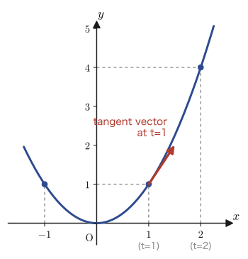
Illustration 17.1: Differentiating $\vec f(t)=[t,t^2]$

An example from the original notes. Consider the graph of $\vec f(t)=[t,t^2]$ (Figure 17.1). Differentiating each component with respect to $t$, we get $x_1'(t)=1$ from $x_1(t)=t$ and $x_2'(t)=2t$ from $x_2(t)=t^2$, so by Definition 17.1

$$ \vec f\,'(t) = [1,\ 2t] $$

For example, the tangent vector at $t=1$ is $\vec f\,'(1)=[1,2]$. It points in the direction obtained by moving one to the right and two up from the point $(1,1)$ at $t=1$ in Figure 17.1 (that is, the direction of a line of slope 2). This agrees perfectly, in terms of direction as well, with the result we learned in high school mathematics that “the slope of the tangent line to $y=x^2$ at $x=1$ is $2\times1=2$.”

Example 17.1: Velocity and speed of a point moving in the plane

Suppose that the position of a point moving in the plane is given at time $t$ (seconds) by $\vec r(t)=[t^2,\,t^3]$ (meters). (a) Find the velocity vector $\vec r\,'(t)$. (b) Find the velocity vector at $t=1$ and the speed at that time (the magnitude of the velocity vector).

Solution. (a) Differentiating component by component according to Definition 17.1, we get $x_1'(t)=2t$ from $x_1(t)=t^2$ and $x_2'(t)=3t^2$ from $x_2(t)=t^3$, so

$$ \vec r\,'(t) = [2t,\ 3t^2]\ \text{(m/s)} $$

(b) Substituting $t=1$ gives $\vec r\,'(1)=[2,3]$ (m/s). The speed is obtained by substituting $t=1$ into the magnitude of the velocity vector, $\abs{\vec r\,'(t)}=\sqrt{(2t)^2+(3t^2)^2}$:

$$ \abs{\vec r\,'(1)} = \sqrt{2^2+3^2} = \sqrt{13}\ \text{(m/s)} $$

(Numerically, $\sqrt{13}\fallingdotseq3.61$.) Note that the velocity vector $\vec r\,'(t)$ is a quantity that has direction as well as magnitude, whereas the speed $\abs{\vec r\,'(t)}$ is a scalar quantity obtained by extracting only its magnitude.

Illustration 17.2: Length of a straight line: $\vec f(t)=[t,2t]$

An example from the original notes. As an example, consider $\vec f(t)=[t,2t]$ (Figure 17.4, the line through the origin with slope 2). Let us find the length from $t=0$ to $t=4$. Since $\vec f\,'(t)=[1,2]$, we have $\abs{\vec f\,'(t)}=\sqrt{1^2+2^2}=\sqrt5$ (a constant independent of $t$), and therefore

$$ S_1 = \int_0^4\abs{\vec f\,'(t)}\,dt = \int_0^4\sqrt5\,dt = \sqrt5\,[\,t\,]_0^4 = 4\sqrt5 $$

Since this curve is a straight line, we can check the result directly with the Pythagorean theorem: the point at $t=0$ is $(0,0)$ and the point at $t=4$ is $(4,8)$, so the distance between the two points is $\sqrt{4^2+8^2}=\sqrt{16+64}=\sqrt{80}=4\sqrt5$, which agrees.

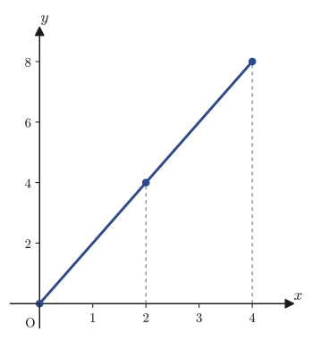
Illustration 17.3: Length of a space curve: $\vec f(t)=[t,\sqrt3\,t,t^2]$

An example from the original notes. Consider $\vec f(t)=[t,\sqrt3\,t,t^2]$. Let us find the length from $t=0$ to $t=\sqrt3$. Since $\vec f\,'(t)=[1,\sqrt3,2t]$, we have

$$ \abs{\vec f\,'(t)} = \sqrt{1^2+(\sqrt3)^2+(2t)^2} = \sqrt{1+3+4t^2} = 2\sqrt{1+t^2} $$

(We factored out $1+3=4$ and wrote $\sqrt{4(1+t^2)}=2\sqrt{1+t^2}$.) Hence we have

$$ S_2 = \int_0^{\sqrt3}\abs{\vec f\,'(t)}\,dt = 2\int_0^{\sqrt3}\sqrt{1+t^2}\,dt $$

Here, using the formula $\displaystyle\int\sqrt{1+x^2}\,dx=\frac12\left(x\sqrt{1+x^2}+\ln\abs{x+\sqrt{1+x^2}}\right)+C$ (a well-known indefinite integral, although it lies outside the scope of high school mathematics; you can verify it yourself with the substitution $x=\tan\theta$, or with the substitution obtained by setting $\sqrt{1+x^2}=u-x$), we get

$$ \int_0^{\sqrt3}\sqrt{1+t^2}\,dt = \frac12\left[t\sqrt{1+t^2}+\ln\abs{t+\sqrt{1+t^2}}\right]_0^{\sqrt3} = \frac12\left(\sqrt3\cdot2+\ln(\sqrt3+2)\right) $$

(We used $\sqrt{1+3}=2$.) Finally, we must not forget that this integral is not $S_2$ itself but the inside of the expression that was doubled to make $S_2$; multiplying by 2 once more at the very end, we obtain

$$ S_2 = 2\times\frac12\left(2\sqrt3+\ln(\sqrt3+2)\right) = 2\sqrt3+\ln(\sqrt3+2)\ \bigl(\fallingdotseq4.78\bigr) $$

which is the correct answer.

Example 17.2: Length of a helix

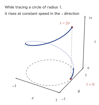
The curve $\vec f(t)=[\cos t,\sin t,t]$ (Figure 17.5) traces a circle of radius 1 in the $xy$-plane while at the same time rising at a constant speed in the $z$ direction; it is called a helix. Picture a spring (coil) or the double-helix structure of DNA. Find the length of this helix from $t=0$ to $t=2\pi$ (exactly one full turn).

Solution. Since $\vec f\,'(t)=[-\sin t,\cos t,1]$, we have

$$ \abs{\vec f\,'(t)} = \sqrt{(-\sin t)^2+(\cos t)^2+1^2} = \sqrt{\sin^2t+\cos^2t+1} = \sqrt{1+1} = \sqrt2 $$

(We used the basic trigonometric identity $\sin^2t+\cos^2t=1$ from high school mathematics.) The speed $\abs{\vec f\,'(t)}=\sqrt2$ is constant, independent of $t$, so the integral is simply a multiplication, and we get

$$ S = \int_0^{2\pi}\sqrt2\,dt = \sqrt2\times2\pi = 2\sqrt2\,\pi\ \bigl(\fallingdotseq8.89\bigr) $$

If there were no rise in the $z$ direction (that is, if it were only the circle in the plane, $\vec f(t)=[\cos t,\sin t]$), the length of one turn would be the circumference $2\pi\times1=2\pi\fallingdotseq6.28$. Since the actual distance traveled along the helix is longer by the amount of the rise, we have $2\sqrt2\,\pi\fallingdotseq8.89>2\pi\fallingdotseq6.28$, which agrees with our intuition.

Example 17.3: Using the integration by parts formula

Let $\vec a(t)=[\sin t,\cos t]$ and $f(t)=t$. Use Formula 17.2(I) to find the indefinite integral $\displaystyle\int t\,\vec a\,'(t)\,dt$.

Solution. We have $\vec a\,'(t)=[\cos t,-\sin t]$. By Formula 17.2(I) ($f=t$, $f'=1$),

$$ \int t\,\vec a\,'(t)\,dt = t\,\vec a(t) - \int 1\cdot\vec a(t)\,dt = t[\sin t,\cos t] - \int[\sin t,\cos t]\,dt $$

Substituting $\displaystyle\int\sin t\,dt=-\cos t+C_1$ and $\displaystyle\int\cos t\,dt=\sin t+C_2$ (basic formulas from high school mathematics), we obtain

$$ \int t\,\vec a\,'(t)\,dt = [\,t\sin t,\ t\cos t\,] - [\,-\cos t,\ \sin t\,] + \vec C = [\,t\sin t+\cos t,\ \ t\cos t-\sin t\,] + \vec C $$

As a check, if we differentiate this result with respect to $t$, the first component becomes $\dfrac{d}{dt}(t\sin t+\cos t)=\sin t+t\cos t-\sin t=t\cos t$, and the second component becomes $\dfrac{d}{dt}(t\cos t-\sin t)=\cos t-t\sin t-\cos t=-t\sin t$. On the other hand, the original integrand is $t\,\vec a\,'(t)=t[\cos t,-\sin t]=[t\cos t,-t\sin t]$, and the two indeed agree.

Example 17.4: Computing a definite integral

Find $\displaystyle\int_0^{\pi}[\cos t,\ \sin t,\ 1]\,dt$.

Solution. Following Definition 17.4, we compute the definite integral component by component.

$$ \int_0^\pi\cos t\,dt = [\sin t]_0^\pi = \sin\pi-\sin0 = 0-0=0 $$ $$ \int_0^\pi\sin t\,dt = [-\cos t]_0^\pi = -\cos\pi-(-\cos0) = -(-1)-(-1) = 1+1=2 $$ $$ \int_0^\pi 1\,dt = [\,t\,]_0^\pi = \pi-0=\pi $$

Therefore,

$$ \int_0^\pi[\cos t,\sin t,1]\,dt = [\,0,\ 2,\ \pi\,] $$

holds.

Example 17.5: Solving a first-order linear differential equation for a vector

Solve the differential equation $\dfrac{d\vec y}{dt}+2\vec y=[\,e^{-2t},\ t,\ 3\,]$ under the initial condition $\vec y(0)=[1,0,0]$.

Solution. Since $p(t)=2$ (a constant), we have $\displaystyle\int p\,dt=2t$, and we solve the equations for the three components, into which the problem decomposes, one at a time by the procedure of Chapter 33 (variation of parameters).

[First component] $y_1'+2y_1=e^{-2t}$. Substituting into Eq. \eqref{eq:17-scalar-ode-solution}, we obtain $y_1(t)=e^{-2t}\left(\displaystyle\int e^{-2t}\cdot e^{2t}\,dt+C_1\right)=e^{-2t}(t+C_1)$. From the initial condition $y_1(0)=1$, we have $1=e^0(0+C_1)=C_1$, so $C_1=1$. Hence $y_1(t)=(t+1)e^{-2t}$.

[Second component] $y_2'+2y_2=t$. The solution of the homogeneous equation $y_2'+2y_2=0$ is $C_2e^{-2t}$. Since the nonhomogeneous term is the polynomial $t$ (of degree 1), we assume a particular solution of the form $y_{2p}=At+B$ ($A,B$ are unknown constants) and substitute it, obtaining $A+2(At+B)=t$, that is, $2At+(A+2B)=t$. Comparing the coefficients of $t$ and the constant terms on the two sides, $2A=1$ gives $A=\dfrac12$, and $A+2B=0$ gives $B=-\dfrac14$. Therefore the general solution is $y_2(t)=\dfrac t2-\dfrac14+C_2e^{-2t}$. From the initial condition $y_2(0)=0$, we have $0=-\dfrac14+C_2$, so $C_2=\dfrac14$. Hence $y_2(t)=\dfrac t2-\dfrac14+\dfrac14e^{-2t}$.

[Third component] $y_3'+2y_3=3$. Since the nonhomogeneous term is a constant, we assume that the particular solution is also a constant, $y_{3p}=k$; then $2k=3$, so $k=\dfrac32$. Adding the homogeneous solution $C_3e^{-2t}$, we obtain the general solution $y_3(t)=\dfrac32+C_3e^{-2t}$. From the initial condition $y_3(0)=0$, we have $0=\dfrac32+C_3$, so $C_3=-\dfrac32$. Hence $y_3(t)=\dfrac32-\dfrac32e^{-2t}$.

Putting these together, the solution is

$$ \vec y(t) = \left[\ (t+1)e^{-2t},\ \ \ \frac t2-\frac14+\frac14e^{-2t},\ \ \ \frac32-\frac32e^{-2t}\ \right] $$

(verified with SymPy's dsolve; see the verification script).

Example 17.6: Parametric representation of a sphere and its partial derivatives

Following the notation for spherical coordinates in Chapter 7, Section 7.7, we express a point on a sphere of radius $R$ using two angles, $\theta$ (the polar angle, measured from the positive direction of the $z$-axis, $0\le\theta\le\pi$) and $\varphi$ (the azimuthal angle, measured from the $x$-axis in the $xy$-plane, $0\le\varphi\lt2\pi$), as

$$ \vec P(\theta,\varphi) = [\,R\sin\theta\cos\varphi,\ \ R\sin\theta\sin\varphi,\ \ R\cos\theta\,] $$

(this expresses the surface that is a sphere as a vector-valued function of the two variables $(\theta,\varphi)$). Find the partial derivatives $\pdiff{\vec P}{\theta}$ and $\pdiff{\vec P}{\varphi}$, and verify that these two vectors are orthogonal to each other.

Solution. Following Definition 17.5, we differentiate each component partially. Differentiating with respect to $\theta$ with $\varphi$ held fixed (using $\dfrac{d}{d\theta}\sin\theta=\cos\theta$ and $\dfrac{d}{d\theta}\cos\theta=-\sin\theta$), we have

$$ \pdiff{\vec P}{\theta} = [\,R\cos\theta\cos\varphi,\ \ R\cos\theta\sin\varphi,\ \ -R\sin\theta\,] $$

Differentiating with respect to $\varphi$ with $\theta$ held fixed (only the factors $\cos\varphi,\sin\varphi$ depend on $\varphi$), we have

$$ \pdiff{\vec P}{\varphi} = [\,-R\sin\theta\sin\varphi,\ \ R\sin\theta\cos\varphi,\ \ 0\,] $$

Computing the inner product of these two vectors, we obtain

$$ \pdiff{\vec P}{\theta}\cdot\pdiff{\vec P}{\varphi} = R\cos\theta\cos\varphi\cdot(-R\sin\theta\sin\varphi) + R\cos\theta\sin\varphi\cdot R\sin\theta\cos\varphi + (-R\sin\theta)\cdot0 $$ $$ = -R^2\sin\theta\cos\theta\cos\varphi\sin\varphi + R^2\sin\theta\cos\theta\sin\varphi\cos\varphi + 0 = 0 $$

(the first and second terms are the same expression differing only in sign, so they cancel exactly when added). Thus indeed $\pdiff{\vec P}{\theta}\perp\pdiff{\vec P}{\varphi}$. This corresponds to the fact that on the sphere, the meridians (the lines along which $\varphi$ is constant and $\theta$ varies) and the parallels of latitude (the lines along which $\theta$ is constant and $\varphi$ varies) intersect at right angles at every point (if you picture a globe, you will find it intuitively convincing that the meridians and parallels are always orthogonal).

Example 17.7: Surface area of a sphere (from the parametric representation)

Using the parametric representation of the sphere from Example 17.6, $\vec P(\theta,\varphi)=[R\sin\theta\cos\varphi,R\sin\theta\sin\varphi,R\cos\theta]$ ($0\le\theta\le\pi$, $0\le\varphi\lt2\pi$), find the surface area of the sphere from Formula 17.3, and verify that it equals $4\pi R^2$.

Solution. We compute the cross product of $\pdiff{\vec P}{\theta}=[R\cos\theta\cos\varphi,R\cos\theta\sin\varphi,-R\sin\theta]$ and $\pdiff{\vec P}{\varphi}=[-R\sin\theta\sin\varphi,R\sin\theta\cos\varphi,0]$, obtained in Example 17.6, according to the component formula for the cross product (let $\vec u=\pdiff{\vec P}{\theta}$ and $\vec v=\pdiff{\vec P}{\varphi}$).

$$ \text{First component:}\ u_2v_3-u_3v_2 = R\cos\theta\sin\varphi\cdot0-(-R\sin\theta)\cdot R\sin\theta\cos\varphi = R^2\sin^2\theta\cos\varphi $$ $$ \text{Second component:}\ u_3v_1-u_1v_3 = (-R\sin\theta)(-R\sin\theta\sin\varphi)-R\cos\theta\cos\varphi\cdot0 = R^2\sin^2\theta\sin\varphi $$ $$ \text{Third component:}\ u_1v_2-u_2v_1 = R\cos\theta\cos\varphi\cdot R\sin\theta\cos\varphi-R\cos\theta\sin\varphi\cdot(-R\sin\theta\sin\varphi) = R^2\sin\theta\cos\theta(\cos^2\varphi+\sin^2\varphi) = R^2\sin\theta\cos\theta $$

(In the last step for the third component, we simplified using $\cos^2\varphi+\sin^2\varphi=1$.) Hence

$$ \pdiff{\vec P}{\theta}\times\pdiff{\vec P}{\varphi} = \left[\,R^2\sin^2\theta\cos\varphi,\ \ R^2\sin^2\theta\sin\varphi,\ \ R^2\sin\theta\cos\theta\,\right] $$

(Verified with SymPy by expansion and simplification.) Its magnitude is

$$ \left|\pdiff{\vec P}{\theta}\times\pdiff{\vec P}{\varphi}\right| = \sqrt{R^4\sin^4\theta\cos^2\varphi+R^4\sin^4\theta\sin^2\varphi+R^4\sin^2\theta\cos^2\theta} = R^2\sqrt{\sin^4\theta(\cos^2\varphi+\sin^2\varphi)+\sin^2\theta\cos^2\theta} $$ $$ = R^2\sqrt{\sin^4\theta+\sin^2\theta\cos^2\theta} = R^2\sqrt{\sin^2\theta(\sin^2\theta+\cos^2\theta)} = R^2\sqrt{\sin^2\theta} = R^2\sin\theta $$

(The last equality holds because $\sin\theta\ge0$ in the range $0\le\theta\le\pi$, so that $\sqrt{\sin^2\theta}=\sin\theta$.) Substituting this into Formula 17.3, we get

$$ S = \int_0^{2\pi}\!\!\int_0^{\pi} R^2\sin\theta\,d\theta\,d\varphi = R^2\left(\int_0^\pi\sin\theta\,d\theta\right)\left(\int_0^{2\pi}d\varphi\right) = R^2\times[-\cos\theta]_0^\pi\times2\pi = R^2\times2\times2\pi = 4\pi R^2 $$

We have thus confirmed that the surface area $4\pi R^2$ of the sphere, obtained in Example 7.13 of Chapter 7, Section 7.7, from the formula for the form $z=f(x,y)$, agrees exactly with the result of the method of this section, which starts from the parametric representation.

Exercise 17.1: Differentiation of vector-valued functions

For $\vec f(t)=[\,t^3-t,\ e^{2t},\ \ln(t+1)\,]$, find the derivative $\vec f\,'(t)$, and then find the tangent vector $\vec f\,'(0)$ at $t=0$.

Hint: Following Definition 17.1, simply differentiate component by component. To differentiate $\ln(t+1)$, use the chain rule (Chapter 3).

→ Solution

Exercise 17.2: Length of a helix

For $\vec f(t)=[\,3\cos t,\ 3\sin t,\ 4t\,]$ (a helix of radius 3), find the length from $t=0$ to $t=2\pi$.

Hint: Use Eq. \eqref{eq:17-arclength} of Definition 17.2. Observe that $\abs{\vec f\,'(t)}$ is a constant independent of $t$.

→ Solution

Exercise 17.3: Computing a definite integral

Find $\displaystyle\int_0^1\left[\,t^2,\ e^t,\ \frac1{1+t^2}\,\right]dt$.

Hint: Compute the definite integral component by component. For the third component, run the differentiation formula for the inverse tangent function $\tan^{-1}t$ (Chapter 3) in reverse.

→ Solution

Exercise 17.4: Applying the integration by parts formula

Let $\vec a(t)=[\,e^t,\ t^2\,]$ and $f(t)=t$. Use Formula 17.2(I) to find $\displaystyle\int t\,\vec a\,'(t)\,dt$.

Hint: We have $\vec a\,'(t)=[e^t,2t]$. Substitute directly into Formula 17.2(I) and compute $\displaystyle\int\vec a(t)\,dt$ (the component-by-component indefinite integral).

→ Solution

Exercise 17.5: A first-order linear differential equation for a vector (a case where resonance occurs)

Solve $\dfrac{d\vec y}{dt}+3\vec y=[\,1,\ t,\ e^{-3t}\,]$ under the initial condition $\vec y(0)=[0,0,1]$.

Hint: For the first and second components, the same procedure as in Example 17.5 works. The third component satisfies $y_3'+3y_3=e^{-3t}$, in which the solution $e^{-3t}$ of the homogeneous equation and the nonhomogeneous term $e^{-3t}$ have the same form (resonance), so we must assume a particular solution of the form $At\,e^{-3t}$ (rather than a constant multiple of the exponential).

→ Solution

Exercise 17.6: Lateral area of a cylinder

The lateral surface of a cylinder of radius $a$ and height $h$ is given by the parametric representation $\vec P(u,v)=[\,a\cos u,\ a\sin u,\ v\,]$ ($0\le u\lt2\pi$, $0\le v\le h$). Use Formula 17.3 to find the lateral area, and verify that it agrees with the familiar formula $2\pi ah$ (circumference of the base circle $\times$ height).

Hint: Find $\pdiff{\vec P}{u}$ and $\pdiff{\vec P}{v}$, and compute the magnitude of the cross product $\pdiff{\vec P}{u}\times\pdiff{\vec P}{v}$.

→ Solution

Exercise 17.7: Why does the cross product point in the normal direction of the surface? (Reasoning from the figure)

Looking at Figure 17.7, explain, on the basis of the figure and the definition of the cross product (Chapter 15), why the cross product $\pdiff{\vec P}{u}\times\pdiff{\vec P}{v}$ of the two tangent vectors $\pdiff{\vec P}{u}\Delta u$ and $\pdiff{\vec P}{v}\Delta v$ that form the infinitesimal area element points in the normal direction (the direction perpendicular to the surface) of the surface $\vec P(u,v)$. No computation is needed.

Hint: The small parallelogram spanned by the two tangent vectors (the filled part of Figure 17.7) approaches, in the limit $\Delta u,\Delta v\to0$, the tangent plane itself (the plane in which the total differential $d\vec P$ moves) at the point $\vec P(u,v)$ on the surface. Recall that the definition of the cross product (Chapter 15) was “the direction perpendicular to both of the two vectors.”

→ Solution