Chapter 8Matrices and Determinants

8.1 Basic Operations on Matrices and Patterns in Matrix Powers

8.1.1 What is a matrix?—A review of matrix operations

An arrangement of numbers in a rectangle is called a matrix. For example,

is a matrix with two rows (running horizontally) and three columns (running vertically). In general, a matrix with $m$ rows (horizontally) and $n$ columns (vertically) is called a matrix of type $(m,n)$, and the number in the $i$th row and the $j$th column is called the $(i,j)$ entry and written $a_{ij}$ (we call $i$ the row index and $j$ the column index. Here an “index” is a subscript: a small number written at the lower right or upper right of a letter). In the example above, $a_{11}=1$ and $a_{23}=2$. In this book, matrices are denoted by capital letters such as $A,B,C,\ldots$.

Calculations with matrices are a straightforward extension of the calculations with numerical vectors that you learned in high school mathematics. For two matrices $A=(a_{ij})$ and $B=(b_{ij})$ of the same type, we define the sum and the scalar multiple as follows.

The real issue is the product. Matrix multiplication does not mean “multiplying the entries in the same positions”; it follows a more intricate rule. Let us first check this with concrete numbers. Take a $2\times3$ matrix $A$ and a $3\times2$ matrix $B$, namely

The $(1,1)$ entry of the product $AB$ is formed from the first row $(1,2,-1)$ of $A$ and the first column $\begin{bmatrix}2\\1\\3\end{bmatrix}$ of $B$ by “multiplying the corresponding entries in order and adding everything up”: $1\times2+2\times1+(-1)\times3=2+2-3=1$. Similarly, the $(1,2)$ entry is obtained from the first row of $A$ and the second column $\begin{bmatrix}0\\-1\\1\end{bmatrix}$ of $B$ as $1\times0+2\times(-1)+(-1)\times1=0-2-1=-3$. The $(2,1)$ entry is obtained from the second row $(0,3,2)$ of $A$ and the first column of $B$ as $0\times2+3\times1+2\times3=9$, and the $(2,2)$ entry from the second row of $A$ and the second column of $B$ as $0\times0+3\times(-1)+2\times1=-1$. Putting these together, we obtain

This is a $2\times2$ matrix. The next definition generalizes this rule of computing by pairing “a row of $A$” with “a column of $B$.”

8.1.2 The transpose

Let us consider the operation of interchanging the rows and columns of a matrix.

For a square matrix, it is easiest to think of the transpose as the operation of “reflecting across the diagonal running from the upper left to the lower right (the diagonal entries, meaning $a_{11},a_{22},a_{33}$).” The entries on the diagonal do not move at all, so their values do not change under transposition. Figure 8.1 shows this.

The transpose has useful properties that we will use repeatedly in later chapters. In particular, transposing the product of two matrices gives the product of their transposes in reverse order. This is not written in the original notes, but since it is a fact used very often when working with matrices, we confirm it here.

8.1.3 Decomposing into column vectors—a computational technique

When working with matrices, taking the viewpoint of “extracting each column as a vector” can sometimes make a computation easier to follow. Let us consider the difference between the following two expressions. Let the columns of $A=\begin{bmatrix}a_{11}&a_{12}&a_{13}\\a_{21}&a_{22}&a_{23}\\a_{31}&a_{32}&a_{33}\end{bmatrix}$ be the column vectors $\vec{x}_1=\begin{bmatrix}a_{11}\\a_{21}\\a_{31}\end{bmatrix}$, $\vec{x}_2=\begin{bmatrix}a_{12}\\a_{22}\\a_{32}\end{bmatrix}$, $\vec{x}_3=\begin{bmatrix}a_{13}\\a_{23}\\a_{33}\end{bmatrix}$. Then the following two expressions, which we build using the real numbers $\lambda_1,\lambda_2,\lambda_3$, look similar but are entirely different in both meaning and type.

(A note on notation: in this chapter we use the symbols $\vec{x}_1,\vec{x}_2,\vec{x}_3$ with arrows to denote “column vectors, that is, numbers arranged vertically.” In Part II (Linear Algebra), even for the same object, a “column vector,” the symbol used for it may be decorated differently from chapter to chapter—for example, some chapters from Chapter 9 onward use the boldface $\bm{x}$. In every case the object referred to (an element of $\R^n$) is the same, and whenever the notation differs from one chapter to another, we will say so in the text at that point.)

8.1.4 Patterns in matrix powers

For a square matrix $A$, we write $A^2=AA$, $A^3=AAA$, …, and in general $A^n$ for the product of $n$ copies of $A$, the number of copies being a natural number (we set $A^0=E$, the identity matrix; the symbol $E$ for the identity matrix will be used consistently from Chapter 9 onward as well). For a general matrix it is difficult to find a regular form for $A^n$, but for $2\times2$ matrices of special forms, $A^n$ follows a remarkably clean pattern. Here we look at three representative patterns.

8.2 Permutations and Their Signs

To define the determinant in the next section (Section 8.3), we need to be ready to handle the operation of “rearranging” mathematically. For example, an operation such as rearranging the three numbers $1,2,3$ into the order $2,3,1$ is called a permutation. In this section we look in turn at the definition of a permutation, the permutation in the reverse direction (the inverse permutation), and the way of assigning a “sign” (plus or minus) to a permutation (even and odd permutations).

8.2.1 Definition of a permutation

Let us look at a diagram that represents the correspondence between the upper and lower rows by arrows, for a permutation with somewhat more elements, $n=4$. Figure 8.2 shows the correspondence of the permutation $\begin{pmatrix}1&2&3&4\\3&1&2&4\end{pmatrix}$ (“$1$ corresponds to $3$, $2$ to $1$, $3$ to $2$, and $4$ to $4$”) represented by arrows.

Let us count how many permutations there are for each value of $n$.

When $n=2$, there are $2$ permutations, $\begin{pmatrix}1&2\\1&2\end{pmatrix}$ and $\begin{pmatrix}1&2\\2&1\end{pmatrix}$ ($2!=2\times1=2$ permutations in all).

When $n=3$, there are $6$ permutations, $\begin{pmatrix}1&2&3\\1&2&3\end{pmatrix}$, $\begin{pmatrix}1&2&3\\1&3&2\end{pmatrix}$, $\begin{pmatrix}1&2&3\\2&1&3\end{pmatrix}$, $\begin{pmatrix}1&2&3\\2&3&1\end{pmatrix}$, $\begin{pmatrix}1&2&3\\3&1&2\end{pmatrix}$, and $\begin{pmatrix}1&2&3\\3&2&1\end{pmatrix}$ ($3!=3\times2\times1=6$ permutations in all).

In general, there are $n$ ways to choose the destination of $1$, then $n-1$ ways to choose the destination of $2$ from the remaining $n-1$ numbers, and so on; counting in this way, we find that there are exactly $n!$ (the factorial of $n$, read “$n$ factorial”) permutations of degree $n$. This is exactly the same as the idea of permutations in high school mathematics (the total number of ways to arrange $n$ distinct objects in a row).

8.2.2 Inverse permutations

As an example, consider the inverse permutation of $\sigma=\begin{pmatrix}1&2&3&4\\3&1&2&4\end{pmatrix}$ ($1$ corresponds to $3$, $2$ to $1$, $3$ to $2$, and $4$ to $4$). If we change “A corresponds to B” into “B corresponds to A,” then $3$ corresponds to $1$, $1$ to $2$, $2$ to $3$, and $4$ to $4$. Hence the inverse permutation of $\sigma$ is $\begin{pmatrix}1&2&3&4\\2&3&1&4\end{pmatrix}$.

The procedure for finding the inverse permutation can be organized into the following two steps.

(i) Exchange the upper and lower rows: $\begin{pmatrix}1&2&3&4\\3&1&2&4\end{pmatrix}\ \longrightarrow\ \begin{pmatrix}3&1&2&4\\1&2&3&4\end{pmatrix}$

(ii) Rearrange the natural numbers in the upper row in increasing order (moving the lower row along with them): $\begin{pmatrix}3&1&2&4\\1&2&3&4\end{pmatrix}\ \longrightarrow\ \begin{pmatrix}1&2&3&4\\2&3&1&4\end{pmatrix}$

Figure 8.3 shows these two steps.

8.2.3 Even and odd permutations

The operation of swapping the correspondences of just two numbers in a permutation is called a transposition. For example, starting from $\begin{pmatrix}1&2&3&4\\1&2&3&4\end{pmatrix}$ (the identity permutation: the permutation in which every number corresponds to itself, so that nothing changes) and repeating the operation of swapping two numbers in the lower row several times, we can produce any permutation.

As an example, let us determine whether $\begin{pmatrix}1&2&3&4\\3&1&2&4\end{pmatrix}$ is an even or an odd permutation. Starting from the identity permutation $\begin{pmatrix}1&2&3&4\\1&2&3&4\end{pmatrix}$, we bring the numbers in the lower row closer to the target arrangement little by little using transpositions.

First, swapping $3$ and $1$ in the lower row gives $\begin{pmatrix}1&2&3&4\\1&2&3&4\end{pmatrix}\to\begin{pmatrix}1&2&3&4\\3&2&1&4\end{pmatrix}$. Next, swapping $2$ and $1$ in the lower row gives $\begin{pmatrix}1&2&3&4\\3&2&1&4\end{pmatrix}\to\begin{pmatrix}1&2&3&4\\3&1&2&4\end{pmatrix}$. We have now reached the target permutation, and the number of transpositions is $2$ (an even number). Hence $\begin{pmatrix}1&2&3&4\\3&1&2&4\end{pmatrix}$ is an even permutation.

8.3 Definition of the Determinant

8.3.1 The sign $\sgn$ and the symbol Σ

We define a function that assigns to each permutation a “sign,” either plus ($+1$) or minus ($-1$).

Next, let us also review the symbol $\Sigma$ (sigma, the Greek letter that denotes a sum), which we will use frequently from this section on. The expression $\displaystyle\sum_{k=1}^{n}c_k$ means “add up everything from $c_1$ to $c_n$, letting $k$ run from $1$ to $n$.” In the following Definition 8.9, we omit the index range and simply write $\sum_{\sigma}$ (meaning “sum over all permutations $\sigma$”).

8.3.2 Definition of the determinant

This definition is also called the Leibniz formula, because it originates with the 17th-century German mathematician Gottfried Wilhelm Leibniz (1646–1716) (in fact, Leibniz himself did not publish it in this form, but he is regarded as one of the first to use the idea of the determinant). The condition “one from each row and each column” corresponds to the ways of placing $n$ chess rooks (or the rook-like hisha pieces of shogi) on an $n\times n$ board so that no two of them share a line of attack (the same row or the same column). Figure 8.5 shows all $3!=6$ placements (= permutations) for $n=3$, together with their signs and the corresponding terms.

Using this definition, let us actually write out the determinant $|A|$ of a general square matrix $A=\begin{bmatrix}a_{11}&a_{12}&a_{13}\\a_{21}&a_{22}&a_{23}\\a_{31}&a_{32}&a_{33}\end{bmatrix}$ of order $3$.

8.4 Cofactors and Expansion of Determinants

The Leibniz formula for determinants in Definition 8.9 clearly defines what a determinant is, but as $n$ grows the number of terms increases explosively to $n!$, so the formula is not suited to actual computation. We therefore introduce a method—cofactor expansion—that reduces a determinant of order $n$ to a combination of smaller determinants of order $(n-1)$.

To confirm that this definition is correct, let us find the determinant of $A_1=\begin{bmatrix}a_{11}&a_{12}&a_{13}\\a_{21}&a_{22}&a_{23}\\a_{31}&a_{32}&a_{33}\end{bmatrix}$.

Eq. \eqref{eq:8-cofactor-row1} is the “cofactor expansion along the first row,” but the same holds for any row and any column. The following theorem states this for the general case of order $n$.

8.5 Properties of Determinants

The determinant has four basic properties that make computations much easier. Here we check them for determinants of order $2$, but, as noted in the margin of the original notes, these properties hold in exactly the same way for columns, and they hold not only for order $2$ but also for determinants of order $n$ (the idea of the proof is the same as for the cofactor expansion in Section 8.4, and it generalizes to the case of order $n$).

If we combine these properties, even a large determinant can be evaluated simply by transforming it into “upper triangular” form (all entries below the diagonal are $0$), in the same way as the elimination method for simultaneous equations in high school mathematics, and then computing the product of the diagonal entries. Indeed, the determinant of an upper triangular matrix equals the product of its diagonal entries—this is a convenient fact to remember, and it can be confirmed from the Leibniz formula for determinants in Definition 8.9: since all the entries in the lower triangular part are $0$, choosing any permutation other than the identity permutation $\sigma=\mathrm{id}$ makes a $0$ appear somewhere in the product $a_{1i_1}\cdots a_{ni_n}$ (one is forced to choose an entry from the lower triangle).

8.6 Geometric Meaning of the Determinant

So far we have treated the determinant as an algebraic computational rule that uses the signs of permutations. But the determinant has another face—the face of expressing the size of a figure. What does it mean for the determinant to be $0$, and what does it mean for it not to be $0$? Let us check with concrete numerical values and graphs.

8.6.1 Two dimensions: area

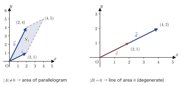
Consider the vectors $\vec{a}=\begin{bmatrix}2\\1\end{bmatrix}$ and $\vec{b}=\begin{bmatrix}2\\4\end{bmatrix}$. Arranging $\vec{a}$ and $\vec{b}$ as columns gives the matrix $A=\begin{bmatrix}2&2\\1&4\end{bmatrix}$.

Computing the determinant, we have

On the other hand, let us find the area $S_1$ of the parallelogram formed by $\vec{a},\vec{b}$ (the left panel of Figure 8.7, with vertices at the origin $O$, the tip $(2,1)$ of $\vec{a}$, the tip $(4,5)$ of $\vec{a}+\vec{b}$, and the tip $(2,4)$ of $\vec{b}$) by subtracting the excess parts from the rectangle that encloses these points. The rectangle enclosing the four points, with exactly two of them as opposite corners, has $x$-range $[0,4]$ and $y$-range $[0,5]$, so its area is $4\times5=20$. The “remainder” left when the parallelogram is removed from this rectangle splits into two small right triangles formed by $\vec a=(a_1,a_2)=(2,1)$ (together equal in area to a rectangle of size $a_1\times a_2$), two right triangles formed by $\vec b=(b_1,b_2)=(2,4)$ (together equal in area to a rectangle of size $b_1\times b_2$), and two rectangles of width $b_1$ and height $a_2$ (in general this decomposition holds when $a_1,b_1>0$ and $0\lt a_2\lt b_2$, and algebraically it corresponds to the identity $(a_1+b_1)(a_2+b_2)=(a_1a_2+b_1b_2)+2a_2b_1+(a_1b_2-a_2b_1)$):

Here $10=a_1a_2+b_1b_2=2\times1+2\times4=2+8$ (the two pairs of right triangles) and $4=2a_2b_1=2\times1\times2$ (the two rectangles). Since Eqs. ① and ② agree, we see that $|A|$ gives the area $S_1$ of the parallelogram.

Now consider another pair, $\vec{c}=\begin{bmatrix}2\\1\end{bmatrix}$ and $\vec{d}=\begin{bmatrix}4\\2\end{bmatrix}$. Putting $\vec c$ and $\vec d$ together gives $B=\begin{bmatrix}2&4\\1&2\end{bmatrix}$. The determinant is

As the right panel of Figure 8.7 shows, $\vec d=2\vec c$ (the same direction, only twice the length), so $\vec c,\vec d$ lie on the same line and no parallelogram is formed (it collapses to a line segment). Hence the area is $0$.

From this we can summarize as follows: in the two-dimensional graph, if the determinant is not $0$, it gives the value of the area, and if it is $0$, the two vectors overlap and a line of area $0$ appears. Let us prove this for a general $2\times2$ matrix.

8.6.2 Three dimensions: volume

Next we consider three dimensions. Consider the vectors $\vec{f}=\begin{bmatrix}1\\2\\3\end{bmatrix}$, $\vec{g}=\begin{bmatrix}2\\-1\\1\end{bmatrix}$, and $\vec{h}=\begin{bmatrix}1\\1\\2\end{bmatrix}$. In fact, these $\vec f,\vec g,\vec h$ all lie in the same plane $S$—that is, they are linearly dependent (one of them can be written as a sum of real multiples of the other two; the rigorous definition is given in Chapter 10). Indeed, the relation $\vec h=\dfrac{3}{5}\vec f+\dfrac{1}{5}\vec g$ holds. Putting $\vec f,\vec g,\vec h$ together as columns gives $C=\begin{bmatrix}1&2&1\\2&-1&1\\3&1&2\end{bmatrix}$. The determinant is

(computed by Sarrus's rule; check this for yourself). Figure 8.8 shows how $\vec f,\vec g,\vec h$ lie in the same plane $S$ (the plane spanned by $\vec f,\vec g$), so that the three vectors from the origin $O$ collapse without forming a parallelepiped.

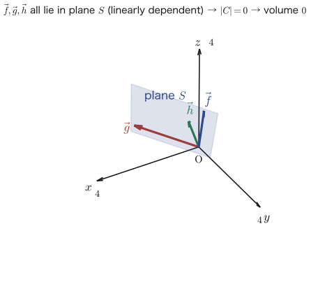
In the three-dimensional graph, if the determinant is not $0$, it gives the value of the volume of the parallelepiped; if it is $0$, the three vectors fit into a single plane, and a plane of volume $0$ appears. As in the two-dimensional case, let us prove the general case. We use the inner product (also called the dot product, $\vec u\cdot\vec v=u_1v_1+u_2v_2+u_3v_3$) that appears in high school mathematics in the study of vectors (vectors in space).

8.7 Summary and Exercises

8.7.1 Summary

• We reviewed matrix addition, scalar multiplication, and multiplication (Definitions 8.2 and 8.3). Matrix multiplication does not satisfy the commutative law ($AB\neq BA$).
• The transpose ${}^{t}A$ (Definition 8.4) is obtained by interchanging rows and columns; ${}^{t}({}^{t}A)=A$ and ${}^{t}(AB)={}^{t}B\,{}^{t}A$ (Theorem 8.1; the transpose of a product reverses the order).
• For the three kinds of matrices—diagonal, upper triangular, and rotation—the powers can be obtained in neat forms (Formulas 8.1–8.3) by mathematical induction. The reason will become clear through diagonalization in Chapter 12.
• A permutation (Definition 8.5) is a rearrangement of $1,\ldots,n$, and there are $n!$ of them in all. The inverse permutation (Definition 8.6) is obtained by exchanging the upper and lower rows and rearranging so that the upper row is in increasing order. Even and odd permutations (Definition 8.7) are determined by the parity of the number of transpositions needed to reach the permutation from the identity permutation, and the sign $\sgn$ (Definition 8.8) is $+1$ for an even permutation and $-1$ for an odd permutation.
• The determinant (Definition 8.9) is the sum of the signed products over all ways of choosing one entry from each row and each column (that is, over all permutations); this is the Leibniz formula for determinants. In the case of order $3$, it coincides with Sarrus's rule (Eq. \eqref{eq:8-det3-sarrus}).
• Using the cofactor $A_{ij}$ (Definition 8.10), the determinant can be computed by cofactor expansion (Theorem 8.2) along any row or any column we like.
• Using the basic properties of determinants (Theorem 8.3)—(i) scalar multiplication of a row, (ii) sign reversal when two rows are interchanged, (iii) invariance when a constant multiple of another row is added, (iv) multilinearity—we can compute even large determinants efficiently, simply by reducing the matrix to upper triangular form and taking the product of the diagonal entries.
• Geometric meaning of the determinant (Theorems 8.4 and 8.5): in two dimensions it equals the area of the parallelogram formed by two vectors, and in three dimensions it equals the volume of the parallelepiped formed by three vectors. That the determinant is $0$ means that the vectors are “squashed” and the dimension drops (that is, they become linearly dependent).

8.7.2 Exercises

8.7.3 References

Related simulator: Determinant (meaning as area and volume)